BIRDFLU Example of sequence statistics and phylogenetic analysis
Contents
Introduction
Spread of Avian Influenza viruses from China to countries has been a great concern recently. Since 2004, hundreds of humans have been infected with bird flu, with about 98 fatalities, mostly in Asia, according to the World Health Organization. It is suspected that the two components of the virus hemagglutinin and neuraminidase molecule are responsible for virulence. In this example we investigate this assumption by considering different segments of the Influenza A virus (H5N1). We also compare segments of H5N1 for several species to investigate the similarity of the virus. Next we compare the virus of one species over different regions to see how the virus is evolved. Comparison are made by phylogenetic analysis.
Load the data in the MATLAB workspace
We consider virus H5N1 (Hong Kong chicken) of 1997 and 2001 and virus H2N3 (ALB mallard duck) of 1985 and 1977. Nucleotide sequences of different segments are collected in FASTA files available here. You can easily read these with the MATLAB function fastaread.
VirusLen=8;

% H5N1 Hong Kong
  s2001 = fastaread('H5N12001Hk.fasta');
  s1997 = fastaread('H5N11997Hk.fasta');

% H2N3 ALB
  t1985 = fastaread('H2N31985Hk.fasta');
  t1977 = fastaread('H2N31977Hk.fasta');
The data correspond to the first coding regions of each segments. They can be also downloaded from the GenBank database.
% data97={ 'H5N11997' 'AF098581' 'AF098594' 'AF098608' 'AF046100' 'AF098620' 'AF098550' 'AF098564' 'AF098573'};
% data01={ 'H5N12001' 'AF509145.1' 'AF509171.1' 'AF509197.1' 'AF509018.1' 'AF509119.1' 'AF509094.1' 'AF509042.1' 'AF509068.1'};
% data85={ 'H2N31985' 'CY003886.1'  'CY003885.1' 'CY003884.1' 'CY003879.1' 'CY003882.1' 'CY003881.1' 'CY003880.1' 'CY003883.1'};
% data77={ 'H2N31977' 'CY003854.1' 'CY003853.1' 'CY003852.1' 'CY003847.1' 'CY003850.1' 'CY003849.1' 'CY003848.1' 'CY003851.1'};
%
% for i=1:VirusLen
%         temp = getgenbank(cell2mat(data97(1,i+1)));
%         temp_seq = temp.Sequence;
%         CDSs = temp.CDS(1);
%         seq1= temp_seq(CDSs.indices(1):CDSs.indices(2));
%         s1997(i).Sequence = fix_seq(seq1(str2num(CDSs.codon_start):end));
%         s1997(i).Header=temp.LocusName;
%         temp = getgenbank(cell2mat(data01(1,i+1)));
%         temp_seq = temp.Sequence;
%         CDSs = temp.CDS(1);
%         seq2= temp_seq(CDSs.indices(1):CDSs.indices(2));
%         s2001(i).Sequence = fix_seq(seq2(str2num(CDSs.codon_start):end));
%         s2001(i).Header=temp.LocusName;
% end
%
% for i=1:VirusLen
%         temp = getgenbank(cell2mat(data77(1,i+1)));
%         t1977(i).Header=temp.LocusName;
%         temp_seq = temp.Sequence;
%         CDSs = temp.CDS(1);
%         seq1= temp_seq(CDSs.indices(1):CDSs.indices(2));
%         t1977(i).Sequence = fix_seq(seq1(str2num(CDSs.codon_start):end));
%         temp = getgenbank(cell2mat(data85(1,i+1)));
%         temp_seq = temp.Sequence;
%         t1985(i).Header=temp.LocusName;
%         CDSs = temp.CDS(1);
%         seq2= temp_seq(CDSs.indices(1):CDSs.indices(2));
%         t1985(i).Sequence = fix_seq(seq2(str2num(CDSs.codon_start):end));
% end
Ka/Ks ratio
We compare corresponding sequences through global alignment and calculate the non-synounymous to synounymous (Ka/Ks) ratio in order to get information on which segment evolves fastest.
% Corrispondence between segments
% Segment 1 = Polymerase (PB2) protein
% Segment 2 = Polymerase (PB1) protein
% Segment 3 = Polymerase (PA) protein
% Segment 4 = Hemagglutinin (HA) gene
% Segment 5 = Nucleocapsid protein (NP) gene.
% Segment 6 = Neuraminidase (NA) gene
% Segment 7 = M1 matrix protein (M) and M2 matrix protein (M) gene
% Segment 8 = Nonstructural /(NS1) protein (NS) gene


 for i=1:VirusLen
    [sc,al] = nwalign(nt2aa(s1997(i).Sequence),nt2aa(s2001(i).Sequence));
    seq1 = seqinsertgaps(s1997(i).Sequence,al(1,:));
    seq2 = seqinsertgaps(s2001(i).Sequence,al(3,:));
    [dn ds vardn vards] = dnds(seq1, seq2);
    DnsH5N1(i) = dn/ds;
 end

 for i=3:VirusLen
    [sc,al] = nwalign(nt2aa(t1985(i).Sequence),nt2aa(t1977(i).Sequence));
    seq1 = seqinsertgaps(t1985(i).Sequence,al(1,:));
    seq2 = seqinsertgaps(t1977(i).Sequence,al(3,:));
    [dn ds vardn vards] = dnds(seq1, seq2);
    DnsH2N3(i) = dn/ds;
 end

DnsH5N1
DnsH2N3
Warning: Proportion of synonymous changes is greater than or equal to 3/4.
Input sequences are too divergent, too short, or contain frame shifts.

d_hat_s =

   NaN

Warning: Proportion of non-synonymous changes is greater than or equal to 3/4.
Input sequences are too divergent, too short, or contain frame shifts.

d_hat_n =

   NaN

Warning: Divide by zero.

DnsH5N1 =

    0.0202    0.0221    0.0280    0.0879    0.0478    0.0931    0.0787       NaN


DnsH2N3 =

         0         0    0.0081    0.0367    0.0067    0.0521       NaN    0.1314
Excluding the last two segments which are very short and therefore not very significant, the segment 6 corresponds to the larger Ka/Ks ratios, i.e. to the segment that evolves faster. Therefore in the following we focus our analysis on that segment only. The second fastest segment seems to be the number 4. This confirms the theory that consider hemagglutin (HA) and neuraminidase (NA) the main responsible for virulence.
Statistical analysis
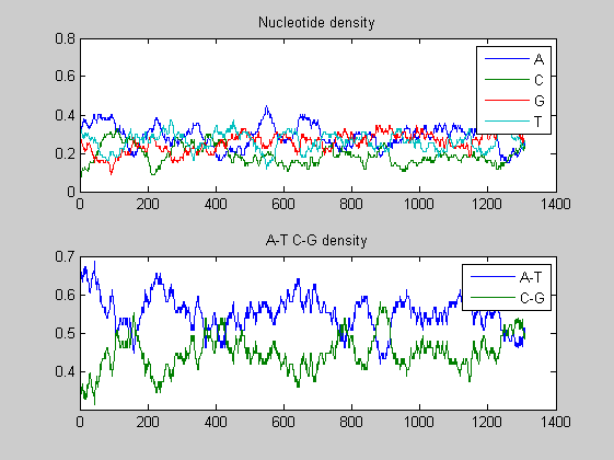
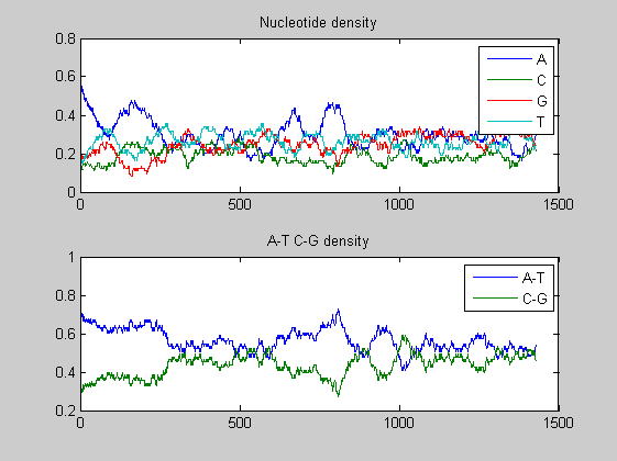
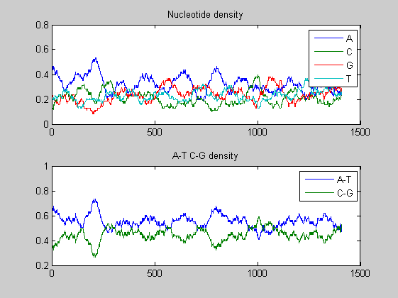
We compare the nucleotide density for both segments in order to see the effect of mutations. The MATLAB function ntdensity can be used for that.
figure
ntdensity(s1997(6).Sequence);
figure;
ntdensity(s2001(6).Sequence);
figure;
ntdensity(t1985(6).Sequence);
figure;
ntdensity(t1977(6).Sequence);
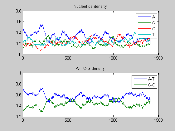
In both viruses the overall trends of the two A-T, C-G densities presents some changes in amplitude as well as in shape highlighting few mutations. We compare also the nucleotide and the dimer composition for both segments of each virus. The functions basecountfrequency and dimercount are used for that.
basecountfrequency(s1997(6).Sequence)
ans =

    A: 380
    C: 249
    G: 336
    T: 343
basecountfrequency(s2001(6).Sequence)
ans =

    A: 429
    C: 268
    G: 352
    T: 379
basecountfrequency(t1985(6).Sequence)
ans =

    A: 456
    C: 296
    G: 332
    T: 326
basecountfrequency(t1977(6).Sequence)
ans =

    A: 468
    C: 280
    G: 321
    T: 341
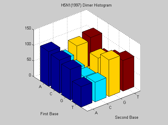
figure;
dimercount(s1997(6).Sequence,'chart','bar');
title('H5N1(1997) Dimer Histogram');
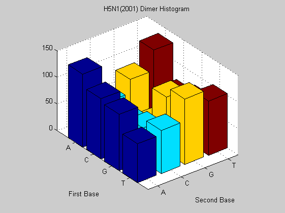
figure;
dimercount(s2001(6).Sequence,'chart','bar');
title('H5N1(2001) Dimer Histogram');
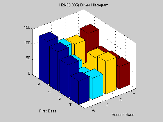
figure;
dimercount(t1985(6).Sequence,'chart','bar');
title('H2N3(1985) Dimer Histogram');
figure;
dimercount(t1977(6).Sequence,'chart','bar');
title('H2N3(1977) Dimer Histogram');
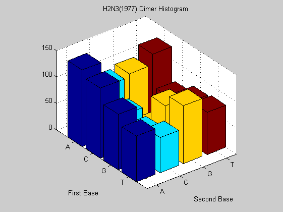
The same virus type from different years shows similar nucleotide and dimer composition. This is more evident in H2N3 while H5N1 changes more in some dimers (i.e. AA, CT). This may explain why it is dreadful nowadays. In fact it has a much faster mutation rate than that of H2N3 even if for the last one there are eight years of difference. To confirm this analysis we also compute the odds for that sequences in order to find unusual dimers.
gss1997=gensign(s1997(6).Sequence)
gss1997 =

    1.0062    0.9546    0.9740    1.0545
    1.4664    1.2456    0.3599    0.9349
    1.0047    0.9075    1.1595    0.8973
    0.6528    0.9656    1.3289    1.0904
gss2001=gensign(s2001(6).Sequence)
gss2001 =

    1.0637    0.8328    0.8801    1.1513
    1.4045    1.1142    0.4847    0.9426
    1.0031    0.9543    1.1994    0.8462
    0.6416    1.1396    1.3175    1.0147
gst1977=gensign(t1977(6).Sequence)
gst1977 =

    0.9277    1.0445    0.9674    1.0875
    1.4213    1.1518    0.3454    0.9162
    0.9862    0.8320    1.1913    0.9797
    0.7604    0.9753    1.4051    0.9708
gst1985=gensign(t1985(6).Sequence)
gst1985 =

    0.9568    1.0663    0.9041    1.0915
    1.3485    1.1434    0.4307    0.9651
    1.0066    0.7753    1.2545    0.9387
    0.7309    1.0089    1.3949    0.9692
Any odds that deviate from 1 are unusually represented. As expected more unusual dimers appears in H5N1 than in H2N3. Furthermore, we count the number of codons for H5N1 genes in the first frame using the MATLAB function codoncount:
frame = 1;
figure;
subplot(2,1,1);
codoncount(s2001(6).Sequence,'frame',frame,'figure',true);
title(sprintf('Codons for Frame %d of H5N1 (2001) Genome',frame));
subplot(2,1,2);
codoncount(s1997(6).Sequence,'frame',frame,'figure',true);
title(sprintf('Codons for Frame %d of H5N1 (1997) Genome',frame));
AAA - 15     AAC - 10     AAG -  7     AAT - 23
ACA -  7     ACC -  7     ACG -  1     ACT - 15
AGA - 10     AGC - 11     AGG -  3     AGT - 14
ATA - 13     ATC - 13     ATG - 10     ATT - 13
CAA -  9     CAC -  3     CAG -  7     CAT -  5
CCA - 11     CCC -  4     CCG -  2     CCT -  6
CGA -  0     CGC -  1     CGG -  2     CGT -  0
CTA -  1     CTC -  1     CTG -  4     CTT -  2
GAA -  9     GAC - 13     GAG - 12     GAT - 11
GCA -  4     GCC -  3     GCG -  1     GCT -  9
GGA - 12     GGC -  9     GGG - 14     GGT -  8
GTA - 11     GTC -  5     GTG -  7     GTT -  7
TAA -  1     TAC -  4     TAG -  0     TAT - 11
TCA - 11     TCC -  6     TCG -  5     TCT -  9
TGA -  0     TGC -  9     TGG - 15     TGT - 10
TTA -  3     TTC - 10     TTG -  9     TTT -  8

AAA - 10     AAC - 10     AAG -  8     AAT - 18
ACA - 11     ACC -  7     ACG -  1     ACT -  8
AGA -  7     AGC - 10     AGG -  8     AGT - 15
ATA - 14     ATC -  9     ATG -  5     ATT - 11
CAA -  7     CAC -  2     CAG -  4     CAT -  6
CCA - 11     CCC -  3     CCG -  2     CCT -  7
CGA -  1     CGC -  1     CGG -  0     CGT -  0
CTA -  3     CTC -  1     CTG -  3     CTT -  1
GAA - 12     GAC - 10     GAG -  9     GAT -  9
GCA -  3     GCC -  4     GCG -  3     GCT -  9
GGA - 11     GGC -  7     GGG - 13     GGT - 10
GTA -  5     GTC -  3     GTG - 10     GTT -  8
TAA -  0     TAC -  8     TAG -  1     TAT -  6
TCA -  9     TCC -  7     TCG -  2     TCT -  9
TGA -  0     TGC - 10     TGG - 16     TGT -  8
TTA -  4     TTC -  9     TTG -  8     TTT -  9
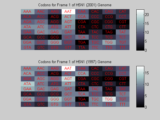
We can see that codon composition is not as similar as the previous counts. There are some subtle changes, for examples, the codon ATA.
Phylogenetic analysis
In this part we first investigate by means of a phylogenetic tree the diffusion of the virus in different places. We consider chicken samples of H5N1 and we perform our analysis only using the segment 5 which we have demonstrated to be the more active. Obviously the same procedure can be repeated for all the other segments.
%        Species Description      GenBank Accession (segment 1 to 8)
%        H5N1
data   = {'Guangdong/2004'        'AY737293' 'AY737294' 'AY737295' 'AY737296' 'AY737297' 'AY737299' 'AY737298' 'AY737300';
           'Kurgan/2005'           'DQ323675' 'DQ323676' 'DQ323674' 'DQ323672' 'DQ323677' 'DQ323673' 'DQ323678' 'DQ323679';
           'HongKong/1997'         'AF098581' 'AF098594' 'AF098608' 'AF046100' 'AF098620' 'AF098550' 'AF098564' 'AF098573';
           'HongKong/2001'         'AF509145' 'AF509171' 'AF509197' 'AF509018' 'AF509119' 'AF509094' 'AF509042' 'AF509068';
           'Henan/2004'            'AY950283' 'AY950276' 'AY950269' 'AY950234' 'AY950255' 'AY950248' 'AY950241' 'AY950262';
           'Hebei/2001'            'DQ351870' 'DQ351874' 'DQ351869' 'DQ343151' 'DQ351864' 'DQ349117' 'DQ351858' 'DQ351863';
           'Hebei/2002'            'DQ351872' 'DQ351873' 'DQ351867' 'DQ343152' 'DQ351866' 'DQ349116' 'DQ351860' 'DQ351861';
           'Hebei/2005'            'DQ351871' 'DQ351875' 'DQ351868' 'DQ343150' 'DQ351865' 'DQ349118' 'DQ351859' 'DQ351862';
           'Jilin/2004'            'AY653193' 'AY653199' 'AY653198' 'AY653200' 'AY653196' 'AY653195' 'AY653194' 'AY653197';
           'Oita/2004'             'AB188813' 'AB188814' 'AB188815' 'AB188816' 'AB188817' 'AB188818' 'AB188819' 'AB188820';
           'Vietnam/2004'          'DQ138178' 'DQ138158' 'DQ099790' 'DQ099760' 'DQ099774' 'DQ094287' 'DQ094265' 'AY770621';
           'Yamaguchi/2004'        'AB166859' 'AB166860' 'AB166861' 'AB166862' 'AB166863' 'AB166864' 'AB166865' 'AB166866';
           };

data_len=size(data,1);

for ind = 1:data_len
    fluh(ind).Header   = data{ind,1};
    fluh(ind).Sequence = getgenbank(data{ind,6},'sequenceonly','true');
end
The data are also available in a .mat file here.
% load fluh6
We compute pairwise distances using the ‘Jukes-Cantor’ formula and the phylogenetic tree with the ‘UPGMA’ distance method. Since the sequences are not pre-aligned, seqpdist will pairwise align them before computing the distances.
distances = seqpdist(fluh,'Method','Jukes-Cantor','Alpha','NT');
Alternate tree topologies are important to consider when analyzing homologous sequences between species. A neighbor-joining tree can be built using the seqneighjoin function. Neighbor-joining trees use the pairwise distance calculated above (using the seqpdist function) to construct the tree.
NJtree = seqneighjoin(distances,'equivar',fluh);
We plot the NJ phylogenetic tree.
h = plot(NJtree,'orient','left');
title(['N.J. Distance Tree of H5N1(chicken) segment 5 using Jukes-Cantor model']);
xlabel('Evolutionary distance')
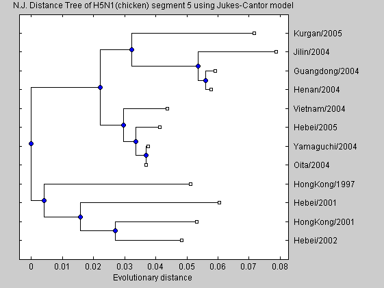
We can see that the recent H5N1 separate from the older virus. It means that this segment evolves over time. Finally, we construct a phylogenetic tree from different species with different virus from different years. This just to show that most of the virus from the same places group together indicating that virus types mutates when they arrive to a different place. As before the analysis is performend with segment 6 sequences.
     %  All Flu
data = {'ALB/H4N3/1977/mallard duck'    'CY004755' 'CY005949' 'CY004754' 'CY005948' 'CY004752' 'CY004751' 'CY004750' 'CY004753';
        'ALB/H12N1/1983/mallard duck'   'CY005350' 'CY005349' 'CY005348' 'CY006006' 'CY005346' 'CY005345' 'CY005344' 'CY005347';
        'ALB/H2N9/1977/pintail duck'    'CY003862' 'CY003861' 'CY003860' 'CY003855' 'CY003858' 'CY003857' 'CY003856' 'CY003859';
        'ALB/H2N3/1977/mallard duck'    'CY003854' 'CY003853' 'CY003852' 'CY003847' 'CY003850' 'CY003849' 'CY003848' 'CY003851';
        'ALB/H2N3/1985/mallard duck'    'CY003886' 'CY003885' 'CY003884' 'CY003879' 'CY003882' 'CY003881' 'CY003880' 'CY003883';
        'ALB/H11N2/1991/mallard'        'CY005311' 'CY005310' 'CY005309' 'CY006003' 'CY005307' 'CY005306' 'CY005305' 'CY005308';
        'ALB/H12N5/1991/grn-winged teal' 'CY005357' 'CY005356' 'CY005355' 'CY006007' 'CY005353' 'CY005352' 'CY005351' 'CY005354';
        'Alberta/H11N9/2000/pintail'    'CY005330' 'CY005329' 'CY005328' 'CY006004' 'CY005326' 'CY005325' 'CY005324' 'CY005327';
        'Colorado/H3N2/1977/swine'      'CY009307' 'CY009306' 'CY009305' 'CY009300' 'CY009303' 'CY009302' 'CY009301' 'CY009304';
        'DE/H12N5/2000/ruddy turnstone' 'CY005371' 'CY005370' 'CY005369' 'CY006008' 'CY005367' 'CY005366' 'CY005365' 'CY005368';
        'DE/H11N9/2003/shorebird'       'CY005337' 'CY005336' 'CY005335' 'CY006005' 'CY005333' 'CY005332' 'CY005331' 'CY005334';
        'Guangdong/H5N1/2004/wild duck' 'AY950284' 'AY950277' 'AY950270' 'AY950235' 'AY950256' 'AY950249' 'AY950242' 'AY950263';
        'HongKong/H3N2/1975/duck'       'CY005559' 'CY005558' 'CY005557' 'CY006026' 'CY005555' 'CY005554' 'CY005553' 'CY005556';
        'HongKong/H4N2/1976/duck'       'CY005631' 'CY005630' 'CY005629' 'CY006030' 'CY005627' 'CY005626' 'CY005625' 'CY005628';
        'HongKong/H6N1/1976/duck'       'CY005604' 'CY005603' 'CY005602' 'CY005597' 'CY005600' 'CY005599' 'CY005598' 'CY005601';
        'HongKong/H4N6/1978/duck'       'CY005574' 'CY005573' 'CY005572' 'CY006027' 'CY005570' 'CY005569' 'CY005568' 'CY005571';
        'HongKong/H5N3/1978/goose'      'CY005589' 'CY005588' 'CY005587' 'CY006028' 'CY005585' 'CY005584' 'CY005583' 'CY005586';
        'HongKong/H5N1/1997/chicken'    'AF098581' 'AF098594' 'AF098608' 'AF046100' 'AF098620' 'AF098550' 'AF098564' 'AF098573';
        'Henan/H5N1/2004/chicken'       'AY950283' 'AY950276' 'AY950269' 'AY950234' 'AY950255' 'AY950248' 'AY950241' 'AY950262';
        'Hidalgo/H5N2/1994/chicken'     'CY005838' 'CY005837' 'CY005836' 'CY006040' 'CY005834' 'CY005833' 'CY005832' 'CY005835';
        'MN/H9N2/1980/goose'            'CY005880' 'CY005879' 'CY005878' 'CY006042' 'CY005876' 'CY005875' 'CY005874' 'CY005877';
        'Nanchang/H3N8/1992/duck'       'CY005475' 'CY005474' 'CY005473' 'CY006016' 'CY005471' 'CY005470' 'CY005469' 'CY005472';
        'Nanchang/H4N6/2000/duck'       'CY005493' 'CY005492' 'CY005491' 'CY006017' 'CY005489' 'CY005488' 'CY005487' 'CY005490';
        'Nanchang/H3N6/2000/quail'      'CY005460' 'CY005459' 'CY005458' 'CY006014' 'CY005456' 'CY005455' 'CY005454' 'CY005457';
        'Nanchang/H9N2/2000/quail'      'CY005506' 'CY005505' 'CY005504' 'CY006018' 'CY005503' 'CY005502' 'CY005501' 'CY006019';
        'Nanchang/H9N2/2001/chicken'    'CY005524' 'CY005523' 'CY005522' 'CY006023' 'CY005521' 'CY005520' 'CY005519' 'CY006024';
        'Potsdam/H5N6/1984/duck'        'CY005776' 'CY005775' 'CY005774' 'CY006036' 'CY005772' 'CY005771' 'CY005770' 'CY005773';
        'Spain/H3N2/2001/swine'         'CY009379' 'CY009378' 'CY009377' 'CY009372' 'CY009375' 'CY009374' 'CY009373' 'CY009376';
        'Spain/H3N2/2002/swine'         'CY009387' 'CY009386' 'CY009385' 'CY009380' 'CY009383' 'CY009382' 'CY009381' 'CY009384';
        'W. Aust./H15N9/1979/w.-tail shearwater' 'CY005412' 'CY005411' 'CY005410' 'CY006010' 'CY005408' 'CY005407' 'CY005406' 'CY005409';
        'W. Aust./H15N9/1983/w.-tail shearwater' 'CY005731' 'CY005730' 'CY005729' 'CY006034' 'CY005727' 'CY005726' 'CY005725' 'CY005728';
        'W. Aust./H15N9/1983/sooty tern' 'CY005724' 'CY005723' 'CY005722' 'CY006033' 'CY005720' 'CY005719' 'CY005718'  'CY005721';
        'Wisconsin/H3N2/1980/swine'     'CY009315' 'CY009314' 'CY009313' 'CY009308' 'CY009311' 'CY009310' 'CY009309' 'CY009312';
        };


for ind = 1:length(data)
    flu(ind).Header   = data{ind,1};
    flu(ind).Sequence = getgenbank(data{ind,6},'sequenceonly','true');
end
The data are also available in a .mat file here.
%load flu6
As before we construct a phylogenetic tree. The distance matrix is computed using the ‘Jukes-Cantor’ correction.
distances = seqpdist(flu,'Method','Jukes-Cantor','Alpha','NT');
We build a neighbor-joining phylogenetic tree and we display it.
NJtree = seqneighjoin(distances,'equivar',flu);
h = plot(NJtree,'orient','left');
title(['N.J. Distance Tree of flu segment 5 using Jukes-Cantor model']);
xlabel('Evolutionary distance')
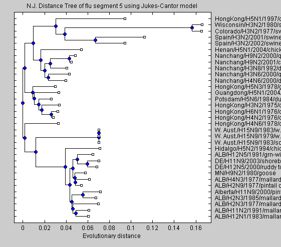
The neighbour joining tree tends to group the virus by location.
References
G. Laver, N. Bischfberger, R.G. Webster, Disarming Flu Viruses, Scientific American Inc., 1998.