SARS Example of phylogenetic analysis
Contents
Introduction
SARS (Severe Acute Respiratory Syndrome) was an illness that first appeared in the second half of 2002 in Guangdong Province (China). The disease is now known to be caused by the SARS coronavirus (SARS CoV), a novel coronavirus. SARS was first reported in Asia (at the Vietnam French Hospital of Hanoi) in February 2003. Over the next few months, the illness spread to several countries all over the world. The origin and diffusion of SARS epidemic is studied in this example. The genome SARS-CoV was completed in April 2003 by a Canadian group of researchers. It is a 29571 base long single stranded RNA sequence. It can be obtained from Genbank database (accession number AY274119.3);
sars_can=getgenbank('AY274119.3','sequenceonly','true');
If you don’t have a live web connection, you can load the data from a MAT-file using the command
%load sars_can % <== Uncomment this if no Internet connection
Finding ORFs
The SARS genome has the typical structure of coronaviruses, with 5 or 6 genes in a caracteristic order. The associated webpage gives some useful information about those genes.
web('http://www.ncbi.nlm.nih.gov/entrez/viewer.fcgi?db=nucleotide&val=30248028');
As observed in the HIV example, the detection of gene in case of viruses is complicated due to overlapping ORFs and other problem. The simplest algorithm to find ORFs in this sequence consists in selecting the statistically significant ORFs between all those found by the function seqorfs. This algorithm can identify most of the genes.
[orf n]=seqorfs(sars_can,'MINIMUMLENGTH',1);
[orfr nr]=seqorfs(sars_can(randperm(length(sars_can))),'MINIMUMLENGTH',1);
ORFLengthr=[];
for i=1:6
    ORFLengthr=[ORFLengthr; orfr(i).Length'];
end
empirical_threshold=prctile(ORFLengthr,95)
[orf n]=seqorfs(sars_can,'MINIMUMLENGTH',empirical_threshold/3);

n
empirical_threshold =

   135


n =

    80
As example we can observe in detail the ORF of the 3rd frame. Let us focus our attention on the sequence between (21492-25257). It coded for the Spike protein that is one of the characteristic gene of coronaviruses. Our following analysis is based on that protein.
SARS_ORF=[orf(3).Start' orf(3).Stop' orf(3).Length' orf(3).Frame']
SARS_ORF =

       13599       21483        7884           3
       21492       25257        3765           3
       25689       26151         462           3
       27273       27639         366           3
       27864       28116         252           3
Reconstructing the Epidemic
During SARS epidemic in 2003 many groups isolated and published the sequence of SARS. Now most of these sequences are available at the Genbank database and can be used to answer many questions about the origin and the nature of epidemic performing genomic sequence analysis.
Identifying the Host
A first question than we can answer about SARS epidemic is related to its origin. The SARS virus was recognized early on as a coronavirus, having the same genes in the same order as other known coronaviruses. However it was very different from any other human coronavirus and hence its origin was likely to be from another animal. Here we compare various animal coronaviruses (including the palm civet). The associated protein sequences can be downloaded from the Genbank database with the MATLAB function getgenpept.
data = {'Bovine CoV1'           'AAL57308.1';
        'Bovine CoV2'           'AAK83356.1';
        'Human CoV OC43'        'NP_937950.1';
        'Porcine HEV3'          'AAL80031';
        'Murine HV1'            'YP_209233.1';
        'Murine HV2'            'NP_045300.1';
        'IBV3'                  'NP_040831.1';
        'Porcine PEDV'          'NP_598310.1';
        'Canine CoV1'           'S41453';
        'Feline CoV4'           'BAA06805';
        'Human Sars CoV'        'AAP41037.1'; % genbank nucleotide id 'AY274119.3';
        'Palm civet'            'AAV49723';
       };


NumCoV=length(data);

for ind = 1:NumCoV
    CoV(ind).Header   = data{ind,1};
    CoV(ind).Sequence = getgenpept(data{ind,2},'sequenceonly','true');
end
Warning: The record 'S41453' has been discontinued in the NCBI database.
Note that the human Sars CoV correspond to the spike protein previously determined with our ORF finding algorithm.
For convenience, the sequence of CoV are also collected in a MAT file and can be load in the workspace.
%load CoV % <== Uncomment this if no Internet connection
We can consider the pairwise distance between sequences with Jukes-Cantor correction and perform the neighbor joining algorithm. The MATLAB function seqpdist can be used for that. Note that this computation is a very time consuming task and can take some minutes.
distances = seqpdist(CoV,'method','jukes-cantor','indels','pairwise-delete','squareform',true);

NJtree = seqneighjoin(distances,'equivar',CoV);
h = plot(NJtree,'orient','left');
title('Neighbor-joining tree using Jukes-Cantor model');
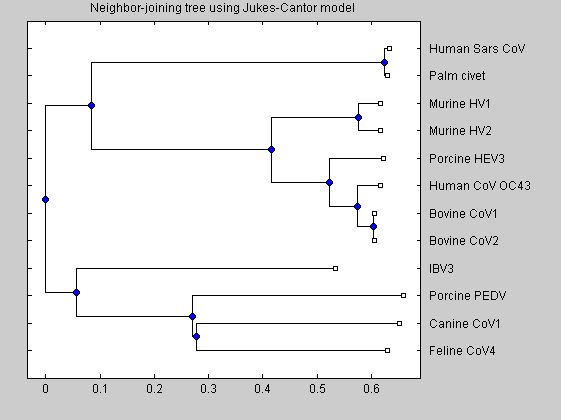
The plot shows the phylogenetic tree. It clearly shows that human SARS is most closely related to Hymalaian palm civet coronavirus and is quite distant from other human coronavirus.
The epidemic tree
We can perform phylogenetic analysis also to reconstruct the diffusion of epidemic between humans. We have chosen 13 sequences for which the date and the location of the sample is known and we used them to perform phylogenetic analysis. They can be obtained from the GenBank database.
sars_data = {   'GZ01'                   'AY278489'       'DEC-16-2002'         'Guangzhou (Guangdong)'    ;
                'ZS-A'                   'AY394997'       'DEC-26-2002'         'Zhongshan (Guangdong)'    ;
                'ZS-C'                   'AY395004'       'JAN-04-2003'         'Zhongshan (Guangdong)'    ;
                'GZ-B'                   'AY394978'       'JAN-24-2003'         'Guangzhou (Guangdong)'    ;
                'HZS-2A'                 'AY394983'       'JAN-31-2003'         'Guangzhou Hospital'       ;
                'GZ-50'                  'AY304495'       'FEB-18-2002'         'Guangzhou (Guangdong)'    ;
                'CUHK-W1'                'AY278554'       'FEB-21-2003'         'Hong Kong'                ;
                'Urbani'                 'AY278741'       'FEB-26-2003'         'Hanoi'                    ;
                'Tor 2'                  'AY274119'       'FEB-27-2003'         'Toronto'                  ;
                'Sin2500'                'AY283794'       'MAR-01-2003'         'Singapore'                ;
                'TW1'                    'AY291451'       'MAR-08-2003'         'Taiwan'                   ;
                'CUHK-AG01'              'AY345986'       'MAR-19-2003'         'Hong Kong'                ;
                'CUHK-L'                 'AY394999'       'MAY-15-2003'         'Hong Kong'                ;
               };

NumSars=size(sars_data,1);
Here we perform our analysis using only the sequences of the spike protein. You can extract them easily from the complete sequences obtained from the Genbank database. Here we show how to do for the first sequence.
sars= getgenbank(sars_data{1,2});
temp_seq = sars(1).Sequence;
CDSs = sars(1).CDS(3);
human_spike(1).Header = CDSs.product;
human_spike(1).Sequence = temp_seq(CDSs(1).indices(1):CDSs(1).indices(2));
For sake of simplicity we have collected them in a FASTA file. You can easily read it with the MATLAB function fastaread
human_spike=fastaread('sars_spike.fasta');

palmcivet_spike=fastaread('spike_palmcivet.fasta');

all_spike=human_spike;
all_spike(NumSars+1).Header=palmcivet_spike.Header;
all_spike(NumSars+1).Sequence=palmcivet_spike.Sequence;
If you don’t have a live web connection, you can load the data from a MAT-file using the command
% load sars_data % <== Uncomment this if no Internet connection
A neighbor joining tree of the Spike protein can be constructed. The distance matrix can be obtained with the Jukes-Cantor corrections on genetic distance calculated from global alignment of the Spike nucleotide sequences.
distances = seqpdist(all_spike,'method','jukes-cantor','alphabet','NT','indels','pairwise-delete','squareform',true);
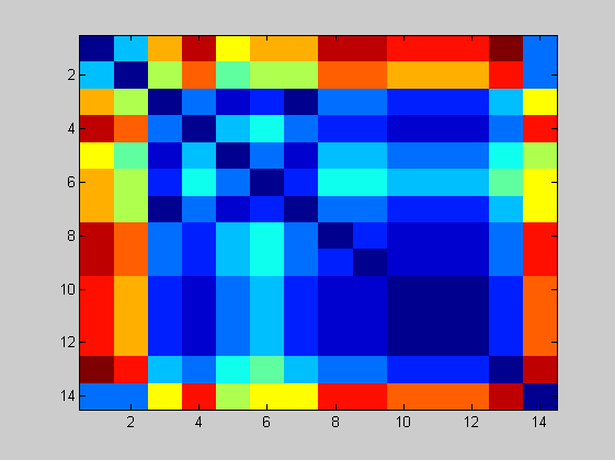
The distance matrix can be also plotted.
figure
imagesc(distances);

NJtree = seqneighjoin(distances,'equivar',all_spike);
h = plot(NJtree,'orient','left');
title('Neighbor-joining tree using Jukes-Cantor model');
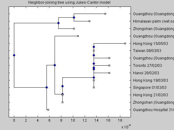
The tree depicts the story of the epidemic. The early infections occurred in the Guangdong province and at the Hotel Metropole: their sequences in fact are very similar. Examining all the branches of the tree we must reconstruct the story of the diffusion of SARS epidemic.
Area of origin
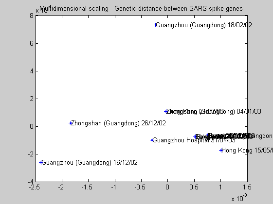
Even if it is known that the first cases of the SARS epidemic appear in the Guangdong province we can study the area of origin of it. The statistical method of multidimensional scaling can be used for that. As previously said in the phylogentic analysis, the area of origin of the virus is in the Guangdong province.
distances = seqpdist(human_spike,'method','jukes-cantor','alphabet','NT','indels','pairwise-delete','squareform',true);
[Y,eigvals] = cmdscale(distances);
figure
plot(Y(:,1),Y(:,2),'*');
for i=1:NumSars
    text(Y(i,1)+.00001,Y(i,2),human_spike(i).Header);
end
title('Multidimensional scaling - Genetic distance between SARS spike genes');
Date of origin
Another question that we can try to answer is related to the date of origin of the epidemic. Knowing the date of each sequence, it is interesting to observe the progression of mutations over time. To do that we first consider the pairwise distance between sequences. Here the Kimura model is used instead of the Jukes-Cantor correction.
distance_Kimura=seqpdist(all_spike,'method','Kimura','squareform',true,'alphabet','NT','indels','pairwise-delete');

for i=1:13
    score(i)=distance_Kimura(14,i);
end

date=[-16 -6 4 24 31 49 52 57 58 60 67 78 135];
plot(date,score,'k*');
hold on;

[P,S] = polyfit(date,score,1);

x=[-150:.1:150];
[y,delta]= polyconf(P,x,S,0.05);
plot(x,y,'b-');
hold on;
plot(x,y+delta,'r-');
hold on;
plot(x,y-delta,'r-');
z=zeros(1,length(x));
hold on;
plot(x,z,'k-');

Relative to the sequence of the palm civet, we see that the genetic distance increases with time in a roughly linear manner. Interpolating in a least-square manner these data, one can approximate date for the origin of the epidemic. Any date compatible with zero distance from the palm civet is a plausible start for the epidemic. We estimate an interval centered around 16 september 2002. The 95% confidence interval are also shown in the plot. Despite its simplicity the method seems to produce correct results because the earliest reported infections dated in the second half of 2002.