SABERTOOTH Example of phylogenetic analysis

Introduction
Statistical analysis
Phylogenetic analysis
Bootstrapping
References

Introduction

America were once home of a huge variety of large felines such as the saber-tooth tigers, the scimitar toothed tigers and the America cheeta-like cats. Only the puma and the jaguar survive today. The saber-tooth and the scimitar toothed tigers and the America cheeta-like cats were species of predators that were extinct about 13000 years ago, towards the end of the last Ice Age. The analysis of the relationship of these old cats and many modern felines is possible thanks to the comparison of the DNA sequences available nowdays. In this example phylogenetic analysis is perfomed and the genetic distances between homologous sequences of different species are calculated. We compare partial cytochrome b sequences of the domestic cat, lion, leopard, tiger, puma, cheetah, African wild cat, Chinese desert cat, and European wild cat with the three extinct species of cats: Smilodon populator, (the saber-tooth tiger), Homotherium (the scimitar toothed tiger) and M. trumani (the American cheetah-like cat).

To perform our analysis we collect all the necessary data in three FASTA files including the corresponding fragments of amino acid and DNA sequences of all the cats obtained with local alignments from the sequences of GenBank. Additionally, there are sequences of other species, added in order to help root the tree and establish proper phylogeny. These are the gray wolf, domestic dog, spotted hyena, striped hyena, black bear, brown bear, and cave bear (now extinct). The FASTA file can be easily accessed with the MATLAB function fastaread

% protein fragments
data = fastaread('catdata.fasta');
% DNA fragments
dnadata = fastaread('catdna.fasta');
% complete cytochrome b sequence of extant cats (all except leopard)
extantdata = fastaread('extantcatdna.fasta');

Statistical analysis

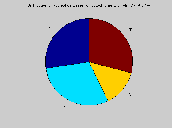
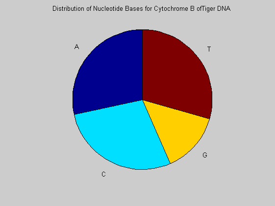
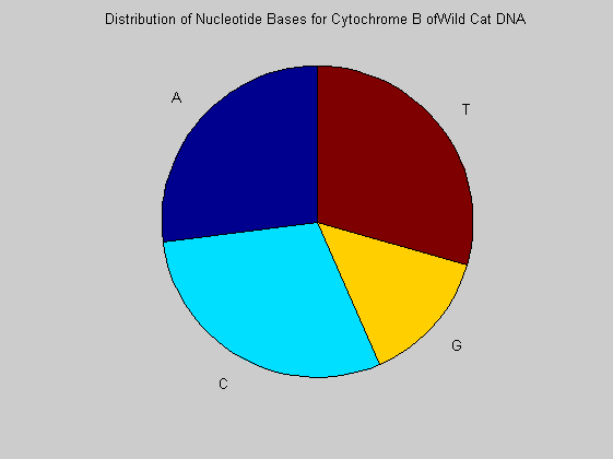
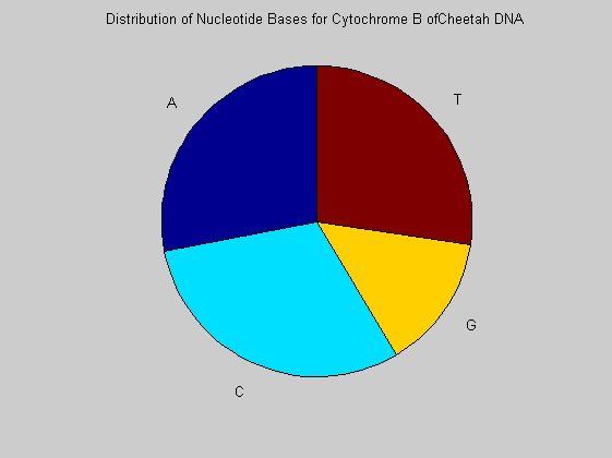
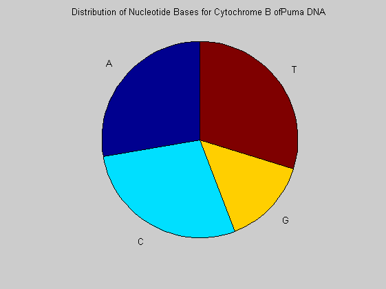
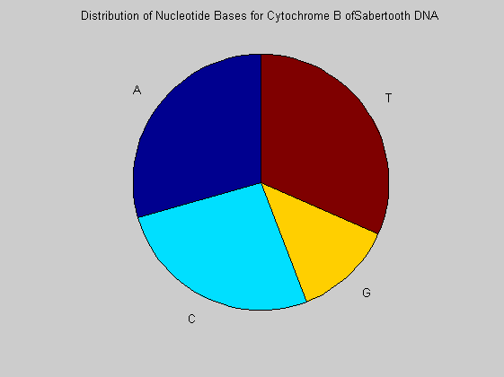
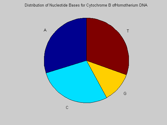
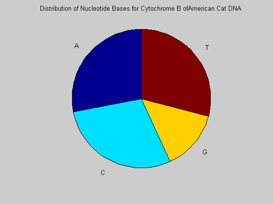
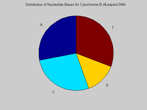
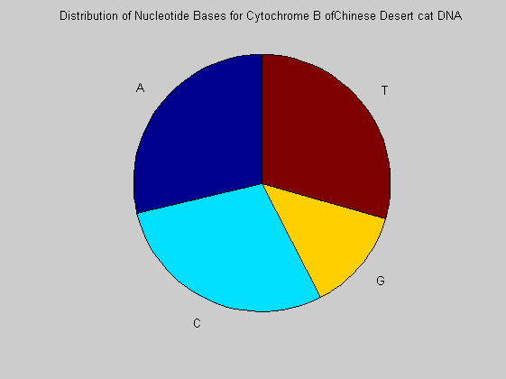
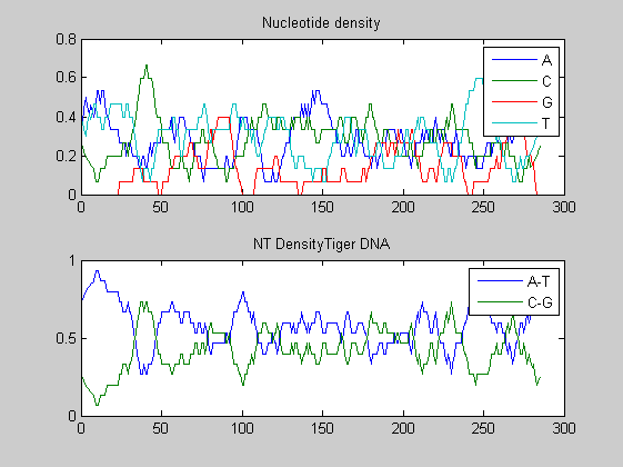
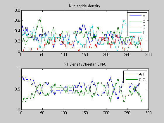
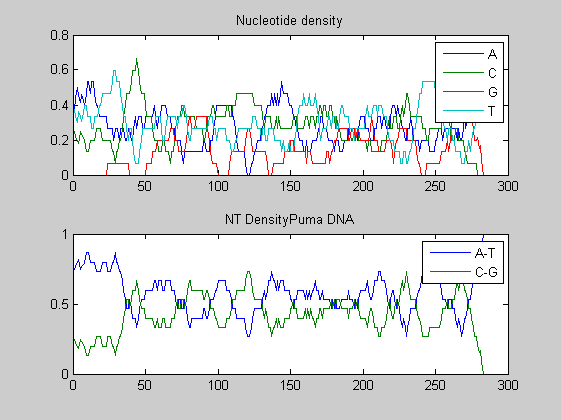
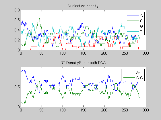
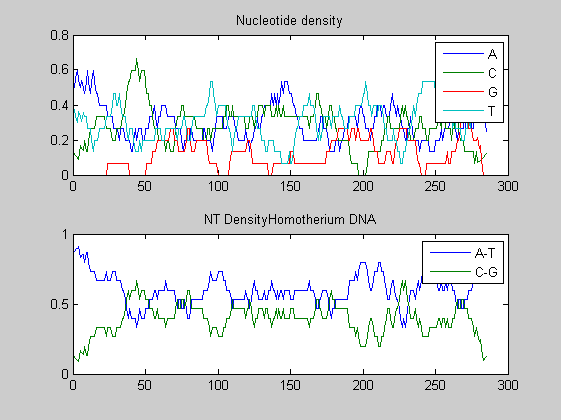
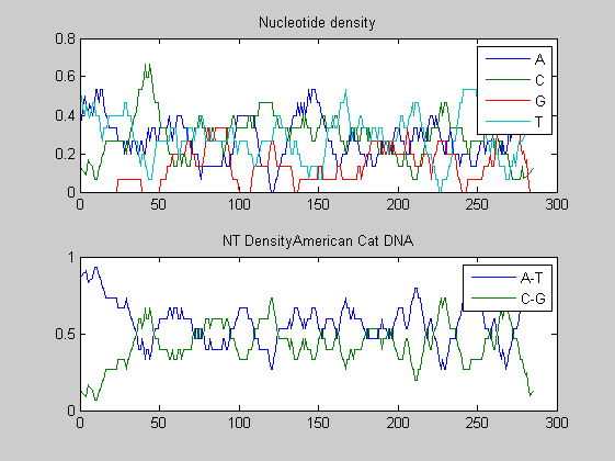
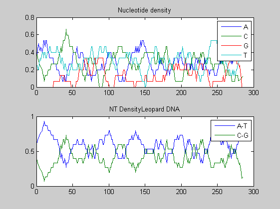
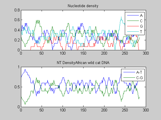
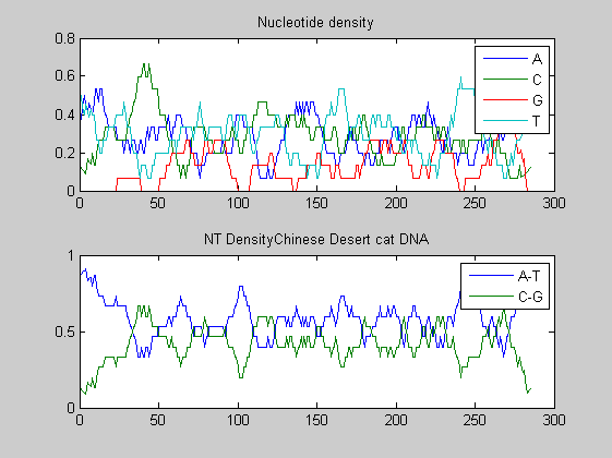
Before performing phylogenetic analysis, we can analyse some statistical properties of the sequences of the cats in order to highlight some meaningful differences between them. First we can count the nucleotides and plots their density.

for i=1:10
    figure
    basecount(dnadata(i).Sequence,'Chart', 'Pie');
    title(strcat('Distribution of Nucleotide Bases for Cytochrome B of',dnadata(i).Header))
end

figure
basecount(dnadata(18).Sequence,'Chart', 'Pie');
title(strcat('Distribution of Nucleotide Bases for Cytochrome B of',dnadata(18).Header))

figure
basecount(dnadata(19).Sequence,'Chart', 'Pie');
title(strcat('Distribution of Nucleotide Bases for Cytochrome B of',dnadata(19).Header))

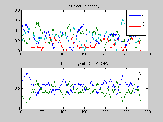
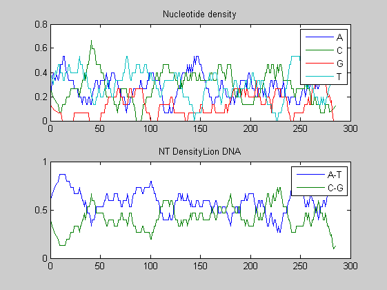
for i=1:10
    figure
    ntdensity(dnadata(i).Sequence);
    title(strcat('NT Density ',dnadata(i).Header))
end

figure
ntdensity(dnadata(18).Sequence);
title(strcat('NT Density ',dnadata(18).Header))

figure
ntdensity(dnadata(19).Sequence);
title(strcat('NT Density ',dnadata(19).Header))

Then we count amino acids in all translated protein fragments.

for i=1:10
    figure
    aacount(data(i).Sequence,'chart','bar');
    title(strcat('Histogram of Amino Acid Count for Cytochrome B of ',data(i).Header));
end

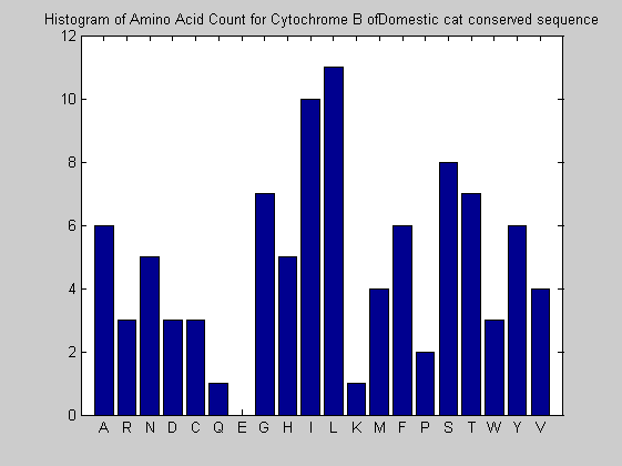
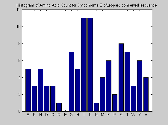
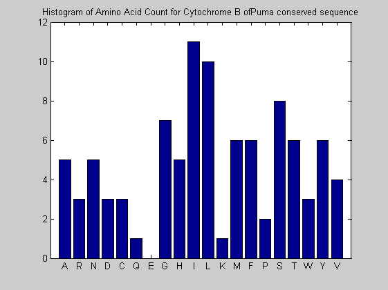
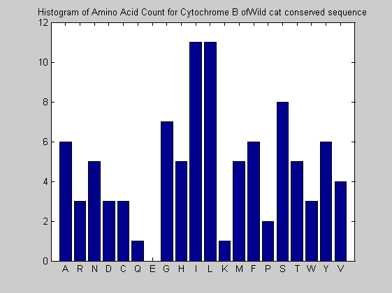
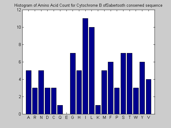
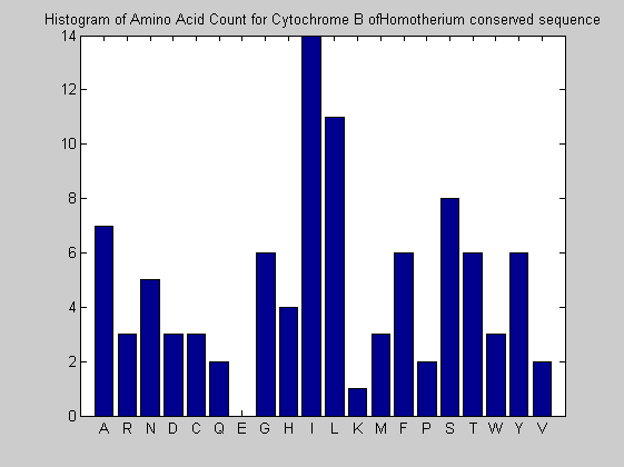
The statistical analysis does not reveal may interesting patterns. GC content varies between all of the species, with some areas of similar base usage and others that are wildly different. The same happens for amino acid content, with variations in the number of each amino acid used in each species.

Phylogenetic analysis

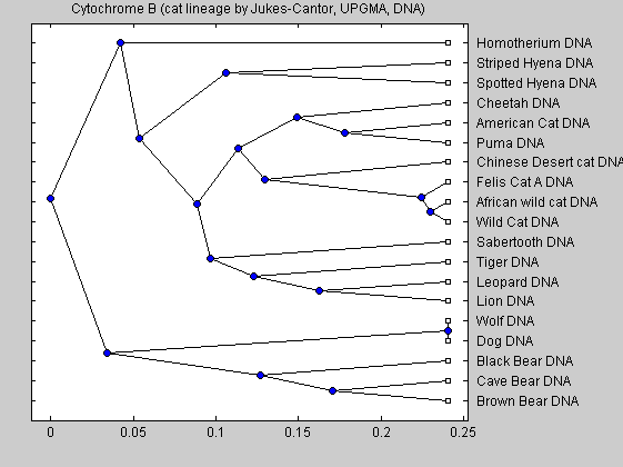
More interesting infomation can be obtained performing phylogentic analysis. We compute the distance matrix with the Jukes-Cantor correction. The MATLAB function seqpdist can be used for that.

catsd = seqpdist(dnadata,'Alphabet','NT');

The phylogenetic tree is constructed with the Unweighted Pair Group Method with Arithmetic Mean (UPGMA) method.

cattreed = seqlinkage(catsd,'UPGMA',dnadata(:,1));
plot(cattreed,'type','angular');
title('Cytochrome B (cat lineage by Jukes-Cantor, UPGMA, DNA)')

We can also look at the tree generated from protein data:

catsnd = seqpdist(data,'method','Alignment','indel','score',...
                    'ScoringMatrix','Blosum62');
catsntree = seqlinkage(catsnd,'UPGMA',data(:,1))
plot(catsntree,'type','angular');
title('Cytochrome B (cat lineage by UPGMA, protein)')

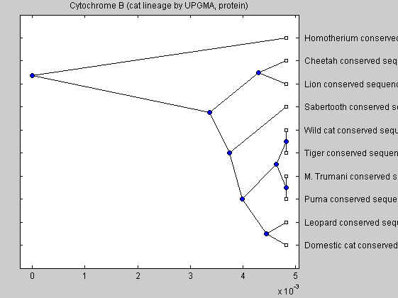
The last tree end up putting the species in a pretty strange order; trees generated from DNA data seem to be more accurrate, so those have been used most.

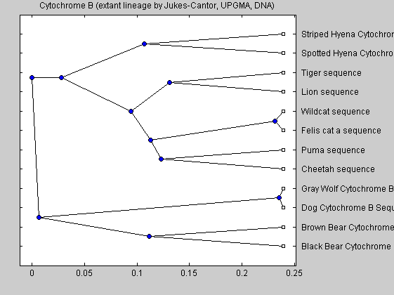
We also consider the tree for extant species only. It is constructed to confirm the to check on how accurate is this method of using full cytochrome b sequence.

extantdata = fastaread('extantcatdna.fasta');
extantsd = seqpdist(extantdata,'Alphabet','NT');
extanttreed = seqlinkage(extantsd,'UPGMA',extantdata(:,1));
plot(extanttreed,'type','angular');
title('Cytochrome B (extant lineage by Jukes-Cantor, UPGMA, DNA)')

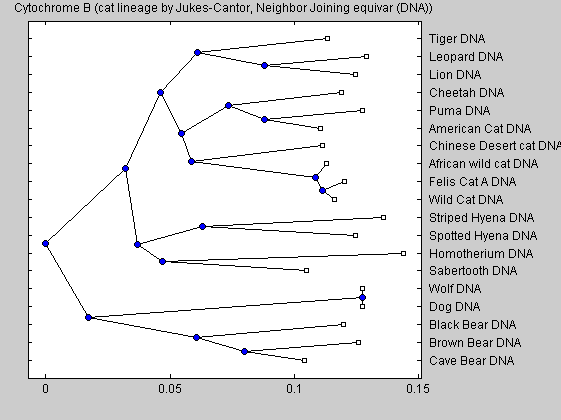
UPGMA and other pairwise alignment methods are older methods for producing trees. The newer and more accurate trees are created by neighbor joining, which is used in the following trees.

cattreed2 = seqneighjoin(catsd,'equivar',dnadata(:,1)); % Assumes equal variance
plot(cattreed2,'type','angular')
title('Cytochrome B (cat lineage by Jukes-Cantor, Neighbor Joining equivar (DNA))')

Bootstrapping

Bootstrap is currently used in the area of evolutionary biology as a tool for both making inferences and for evaluating robustness of some methods. Here we use bootstrap to gives a confidence value for the phylogenetic analysis. 100 bootstrap replicates for each sequence are made, then the distances between those sequences are computed. This is a quite computationally expensive task.

num_seqs = length(dnadata)
num_boots = 100;
seq_len = length(dnadata(1).Sequence);

boots = cell(num_boots,1);
for n = 1:num_boots
    reorder_index = randsample(seq_len,seq_len,true);
    for i = num_seqs:-1:1
        bootseq(i).Header = dnadata(i).Header;
        bootseq(i).Sequence = strrep(dnadata(i).Sequence(reorder_index),'-','');
    end
    boots{n} = bootseq;
end

seq_dists = cell(num_boots,1);
for n = 1:num_boots
     seq_dists{n} = seqpdist(boots{n});
end

num_seqs =

    19

Then the distance information are used to construct trees with the neighbor joining algorithm.

boot_trees = cell(num_boots,1);
 for n = 1:num_boots
      boot_trees{n} = seqneighjoin(seq_dists{n},'firstorder',{dnadata.Header});
 end

Finally the topology of every bootstrap tree is compared with that of the original one to calculate some confidence value for each branch.

for i = num_seqs-1:-1:1
    branch_pointer = i + num_seqs;
    sub_tree = subtree(cattreed2,branch_pointer);
    orig_pointers{i} = getcanonical(sub_tree);
    orig_species{i} = sort(get(sub_tree,'LeafNames'));
end

for j = num_boots:-1:1
    for i = num_seqs-1:-1:1
        branch_ptr = i + num_seqs;
        sub_tree = subtree(boot_trees{j},branch_ptr);
        clusters_pointers{i,j} = getcanonical(sub_tree);
        clusters_species{i,j} = sort(get(sub_tree,'LeafNames'));
    end
end

count = zeros(num_seqs-1,1);
for i = 1 : num_seqs -1
    for j = 1 : num_boots * (num_seqs-1)
        if isequal(orig_pointers{i},clusters_pointers{j})
            if isequal(orig_species{i},clusters_species{j})
                count(i) = count(i) + 1;
            end
        end
    end
end

Pc = count ./ num_boots

[ptrs dist names] = get(cattreed2,'POINTERS','DISTANCES','NODENAMES');

for i = 1 : num_seqs -1
    branch_ptr = i + num_seqs;
    names{branch_ptr} = [names{branch_ptr} ', confidence: ' num2str(100*Pc(i)) ' %'];
end

tr2 = phytree(ptrs,dist,names);
phytreetool(tr2)
plot(tr2)
title('Bootstrapping using Neighbor Joining Tree');

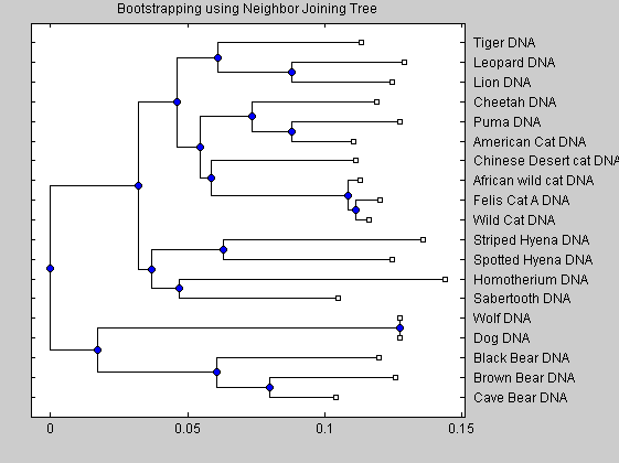
The neighbor joining analysis shows that the American cheetah-like cat is more closer related to the puma than to the true African cheeta. Our analysis is in accordance with the work of Barnett et al. The similar morphological caracteristic of both animals (elongated limbs and enlarged nares) seems therefore the effect of parallel evolutions instead of direct connection. The development of similar bodies caracteristics is due to a similar response in similar ecological pressures. Our analysis shows also that the sabertooth tigers diverged very early on from the ancestors of modern cats and are not closely related to any modern felines.

References

R. Barnett, I. Barnes, M.J. Phillips, L.D. Martin, C.R. Harington, J.A. Leonard, A. Cooper, Evolution of the extinct Sabretooths and the American cheetah-like cat, Curr Biol. Aug 9; vol. 15(15), 2005.

P. Christiansen, J.M. Harris, Body size of Smilodon (Mammalia: Felidae). J Morphol. 266(3):369-84, Dec 2005.

W.E. Johnson,E. Eizirik, J. Pecon-Slattery, W.J. Murphy, A. Antunes, E. Teeling, S.J. O’Brien. The late Miocene radiation of modern Felidae: a genetic assessment. Science. 6;311(5757):73-7, Jan 2006.

O.Loreille, L. Orlando, M. Patou-Mathis, M. Philippe, P. Taberlet, C. Hanni Ancient DNA analysis reveals divergence of the cave bear, Ursus spelaeus, and brown bear, Ursus arctos, lineages. Curr Biol. 6;11(3):200-3, Feb 2001.

L.D. Martin, J.P. Babiarz, V.L. Naples, J. Hearst. Three ways to be a saber-toothed cat. Naturwissenschaften. 87(1):41-4, Jan 2001.

R. Masuda, J.V. Lopez, J.P. Slattery, N. Yuhki, S.J. O’Brien. Molecular phylogeny of mitochondrial cytochrome b and 12S rRNA sequences in the Felidae: ocelot and domestic cat lineages. Mol Phy Evol. 6(3):351-65,1996.