JUKESCANTOR Example of Jukes-Cantor model of a sequence evolution

Contents

Introduction

One of the crucial tasks in computational genomics is represented by the estimation of the genetic distance between two homologous sequences, that is the number of of substitutions that have accumulated between them since they diverged from their common ancestor. The problem is not easy since it means not simply count the number of position at which the two sequence differ. This underestimate the true genetic distance due to multiple substitutions occurred at the same site. To solve this problem, a common approach is to correct the observed genetic distance between two sequences by using a probabilistic model. Several models have been developed in the past. The simplest (the well known Jukes-Cantor model) assumes that each substitution has the same probability. In this demo we show the effect of the JC correction.

Observed genetic distance

Starting with a random sequence of length 1000, you must perform one random substitution at each of the 2000 epochs.

L=1000;
M=2000;

In order to get statistics you may average all over 10 experiments.

R=10;

A random substitution is performed for each experiment every epoch and the difference between the current sequence and the original one are calculated.

for n=1:R
    seq=randseq(L);
    seq1=seq;
    for i=1:M
        j=floor(rand*(L-1))+1;
        seq1(j)=randseq(1);
        v(i,n)=L-length(find((seq-seq1)==0));  %OBSERVED differences
    end
end

Now you can perform some statistics: the mean and the standard deviation of the differences are calculated.

mm=mean(v');
ss=std(v');

Jukes Cantor correction

You must apply the JC correction to the observed differences between the two sequences. An estimate of the genetic distance and of its standard deviation is obtained.

 p=mm/L;
 E=sqrt(p.*(1-p)./(L*((1-(4/3).*p).^2)));
 d = -3/4 * log(1 - p * 4/3);

The error bars for the two cases are computed.

 figure;
 subplot(2,1,1), errorbar(mm,ss)
 title('Simulating the Effect of Multiple Substitutions')
 xlabel('True Number of Substitutions');
 ylabel('Observed Num. of Substitutions')
 subplot(2,1,2), errorbar(d*L,E)
 xlabel('True Number of Substitutions');
 ylabel('Estimated Num. of Substitutions')

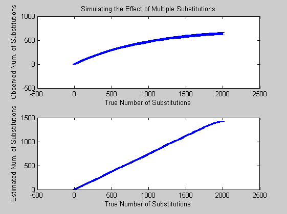
From the plot you may notice that after 2000 substitutions, less than half are actually observable. Moreover applying the JC correction it turns out an almost linear relation between mean and std deviation. This is due to the fact that the JC model consider equal probability of substitution among all symbols.

Published with MATLAB® 7.1