HUMANS Example of sequence comparison by genetic distance

Contents

Introduction

The discovery of Neanderthal skeletons in various parts of Europe raised many questions about human origis, among them the issue of our relation with these species. Now many questions about human and primate origins have been answered by the study of the mitochondrial genome and in particular of the hypervariable regions. These regions presents high sequence variability among humans, therefore they are ideal for studying the relationships among individuals. There are two hypervariable regions called HVR-I and HVR-II.

Load data into MATLAB workspace

In this demostration we first consider the HVR-1 and HVR-2 extracted from Nenderthal bones. Two Neanderthals are considered. The associated sequences can be download from the Genbank database.

% hvr-1
nea_1(1)=getgenbank('AF011222');
nea_1(2)=getgenbank('AF282971');


% hvr-2
nea_2(1)=getgenbank('AF142095');
nea_2(2)=getgenbank('AF282972');

If you don’t have a live web connection you can load them directly into the MATLAB workspace.

% load genbanknean    % <== Uncomment this if no internet connection

The mtDNA sequences of the Neanderthal are compared with 206 mtDNA sequences of modern humans. The complete D-loop is considered for each modern humans. The sequences have been extracted from the Max Ingman database. The associated web page can be explored by the URL.

web('http://www.genpat.uu.se/mtDB');

The data corresponding to both the D-loop are in the FASTA format and can be read using the MATLAB function fastaread.

human_dloop=fastaread('d_loop.fasta');
n=length(human_dloop);

[Note: the d_loop.fasta file can be found here]

Since the sequence of the Neanderthal are incomplete, the corresponding fragments of D-loop of modern human are extracted by local alignment. To this aim the HVR-1 and 2 of the first Neanderthal is considered.

nea.Header='First Neanderthal';
nea.Sequence=strcat(nea_1(1).Sequence,nea_2(1).Sequence);

score=zeros(n,1);
startat=zeros(n,1);

for i=1:n
      [sc,alignment,st]=swalign(human_dloop(i).Sequence,nea.Sequence,'Alphabet', 'NT');
      [m,offset]=size(alignment);                                             % calculate the offset
      startat(i,1)=st(1);                                                     % record the starting index
      endat(i,1)=min(startat(i,1)+offset-1,length(human_dloop(i).Sequence));       % record the ending index
      % the ending index is calculate as minimum between start + offset and length of the sequence because
      % the alignment can produce a lot of gaps
end

real_offset=min(min(endat-startat+1));

The final sequences of humans and Neanderthals are saved in the same structure.

for i=1:n
    hvr_tot(i).Sequence=human_dloop(i).Sequence(startat(i,1):startat(i,1)+real_offset-1);
end

hvr_tot(n+1).Sequence=strcat(nea_1(1).Sequence,nea_2(1).Sequence);
hvr_tot(n+2).Sequence=strcat(nea_1(2).Sequence,nea_2(2).Sequence);

Genetic distances

The genetic distances between each pair of sequences are computed with the Jukes-Cantor correction. It is a very time consuming task, therefore we give also the precomputed matrix. You can load it directly in the workspace.

%distances = seqpdist(hvr_tot,'Method','Jukes-Cantor','Alphabet', 'NT', 'PairwiseAlignment', true);

%D=squareform(distances);

load D

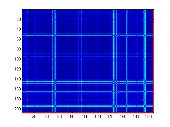
The distance matrix can be plotted. From the image it clearly appears that the zone corresponding to the higher values of distances (red) are those of distances between humans and Neanderthals.

imagesc(D);
legend

We can calculate also the mean distance among any two H. sapiens and between Neanderthal and any modern human.

D_human=reshape((D(1:n,1:n)),1,n^2);
human_dist=mean(D_human(find(D_human>0)))

D_mix=[D(1:n,n+1); D(1:n,n+2)];
mixed_dist=mean(D_mix)

human_dist =

    0.0890


mixed_dist =

    1.0739

The situation can be visualized also through multidimensional scaling, a statistical visualization method that enables us to enbed the datapoints on a plane in a way that respects their pairwise distances.

[Y,eigvals] = cmdscale(D);
plot(Y(1:n,1),Y(1:n,2),'.');
hold on
plot(Y(n+1:n+2,1),Y(n+1:n+2,2),'r*');
title('Relative Distances: 206 H.Sapiens and 2 H.Neanderthalensis');
hold off

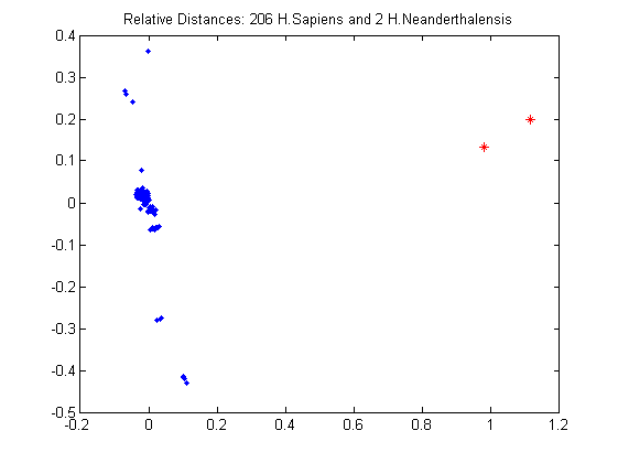
From the plot it is evident that the Neanderthal sequences are very distant to the 206 Homo Sapiens distances. It means that Homo Neanderthalensis were a different species and are very different from modern humans.

Primate evolution

We study the relationship between primates, humans and Neanderthal through phylogenetic analysis. The Hypervariable region II of human, Neanderthal, chimpanzee, bonobo, gorilla, orangutan and gibbon are considered. The genetic distance are estimated as above with the Jukes-Cantor correction.

hvr_primates=fastaread('human_primates_hvr_2.fasta');
distances= seqpdist(hvr_primates,'Method','Jukes-Cantor','Alphabet', 'NT');
tree = seqlinkage(distances,'UPGMA',hvr_primates);

The phylogenetic tree is shown.

h1 = plot(tree,'orient','bottom');
ylabel('Genetic Distance')

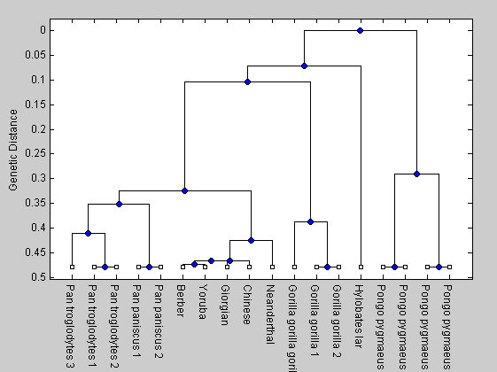
From the tree it is evident that the Neanderthals are more closely related to modern humans than are any of the other primates.
With view you can further explore/edit the phylogenetic tree using an interactive tool.

view(tree)

Published with MATLAB® 7.1