CHLAMYDIA Example of whole genome comparison

Contents

Introduction

Human beings have multiple species of bacteria living within them. Most of these bacteria are not harmful to us and are considered beneficial symbionts. They provide us some benefic effects, for example producing chemicals necessary to our organism. Some symbionts have moved permanently into the cells of their hosts, becoming completely dependent from them. As a consequence of that, their genomes have undergone dramatic changes, losing most part of genes. Therefore intracellular symbiont genomes are some of the smallest known, both in the total size and in the number of genes. In these example the genomes of symbionts of Chlamydia family are examined. In particular we focus our attention on two symbionts: Chlamydia trachomatis (CT) and Chlamydia pneumoniae (CP). They are both intracellular symbionts of humans, also called parasites because they do not provide any benefit to the host. They show a very reduced metabolic and biosynthetic functions and have a very small genome (about 1 Mb length). Here we examine the relationship between them with the typical tools of whole genome comparison. The nucleotide sequences of both parasites can be downloaded from the GenBank database with the MATLAB function getgenbank

CT=getgenbank('NC_000117','sequenceonly','true');

CP=getgenbank('NC_002179','sequenceonly','true');

If you don’t have a live web connection, you can load the data from a MAT-file using the command

%load Chlamydiae    % <== Uncomment this if no internet connection

Comparing ORFs

A first step in our analysis is comparing the genes contained in the Chlamydia genome. Genes in fact serve as landmark in the genome helping the identification of homologous regions between two sequences. Therefore we must identify the ORFs. With the function seqorfs the ORFs longer than 100 codons are selected in both cases.

[orft nt]=seqorfs(CT,'MINIMUMLENGTH',100);

nt

[orfp np]=seqorfs(CP,'MINIMUMLENGTH',100);

np

nt =

   916


np =

        1048

There is only a slight difference in the number of genes between the two genomes, with Chlamydia pneumoniae having about 100 more genes.

Identifying orthologous and paralogous genes

The following step in genome comparison is to compare genes that have been lost or gained between the two parasites. This requires to consider all possible pairs of genes. To do that, a simple approach is to construct a matrix of similarity scores between all the possible pairs of genes of the sequences. We consider the amino acid sequence of every ORF and for each pair of ORFs we compute the Needleman-Wunsch global alignment score. For simplicity, after removing symbols different from A, T, C and G, the two nucleotide sequences are joined together and the orfs are considered in the joined sequence and in its reverse complement. Then they are converted into the associated amino acid sequence and the score matrix is computed.

joined = joinseq(CT,CP);

joined = fix_seq(joined);

orft = seqorfs(joined, 'MINIMUMLENGTH', 100);

seq1_orfs=[];
for i=1:6
     seq1_orfs=[seq1_orfs; orft(i).Start' orft(i).Stop' orft(i).Length' orft(i).Frame'];
end

The computation of the matrix is a quite demanding task since it require to perform several alignment. You can simply load it from a MAT-file using the command

 load Chlamydia_ORFs_similarity.mat

% seq1_orfs=sortrows(seq1_orfs);
% seq1=joined;
% seq2=seqrcomplement(joined);
% for ii=1:length(seq1_orfs)
%     if seq1_orfs(ii,4)>0
%         s=nt2aa(seq1(seq1_orfs(ii,1):seq1_orfs(ii,2)));
%     else
%         s=nt2aa(seq2(seq1_orfs(ii,1):seq1_orfs(ii,2)));
%     end
%     for jj=1:length(seq1_orfs)
%         if seq1_orfs(jj,4)>0
%             t=nt2aa(seq1(seq1_orfs(jj,1):seq1_orfs(jj,2)));
%         else
%             t=nt2aa(seq2(seq1_orfs(jj,1):seq1_orfs(jj,2)));
%         end
%         matrix(ii,jj)=nwalign(s,t);
%     end
% end

The similarity matrix can be used to distinguish between orthologous and paralogous genes. Here we identify Best Reciprocal similarity Hits (BRHs): pair of ORFs that are each other’s best match between two genomes using alignment-based genetic distances.

[ortho para orthoCT orthoCP paraCT paraCP]= brh(matrix)

ortho =

   728


para =

   126


orthoCT =

   401


orthoCP =

   327


paraCT =

    56


paraCP =

    70

We find 728 pairs of orthologous genes (401 in CT and 327 in CP) and 127 pairs of paralogous genes (66 in CT and 71 in CP).

Identifying gene families

In general gene family are groups of closely related genes that have similar function because they share a similar ancestor. In this example we want identify equivalent gene families across the two genomes of CT and CP.

seq1_orfs = fix_seqorfs(seq1_orfs, length(joined));


% this formats the distance matrix a bit
mat1=matrix+min(min(matrix));
mat2=max(max(mat1))-mat1;
mat3=mat2-diag(diag(mat2));

Then we cluster the genes with hierarchical clustering and plot the results.

X=linkage(squareform(mat3));
T=cluster(X,'maxclust',1000);
figure;
barh(sort(hist(T,1000), 'descend'))
title('Gene family size distribution in Chlamydia')
xlabel('Family Size')
ylabel('Number of Gene Families')

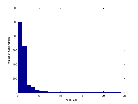
There is a large number of small gene families and a small number of large ones. We can analyze the elements of each cluster and its size. For example let us analyze the largest cluster.

for i=1:length(T)
    cluster{i}.elements=find(T==i);
    clu_size(i)=length(cluster{i}.elements);
end


largest_family=find(clu_size == max(clu_size))
cluster{largest_family}.elements

largest_family =

     6


ans =

          72
         139
         161
         184
         205
         206
         422
         620
         676
         708
         712
         713
         938
         968
         974
         976
        1118
        1312
        1409
        1424
        1447
        1448
        1458
        1931

For each cluster we can recover the coordinates of the ORFs and their sequences. We save them in a FASTA file. From it we can blast them to identify the protein family. The same procedure can be repeated also for other clusters.

FAM_ORFs=seq1_orfs(cluster{largest_family}.elements,:);

for i=1:length(FAM_ORFs)
    seq(i).Header=strcat('FAM1_',char(64+i));
    if (FAM_ORFs(i,4)>0)
        seq(i).Sequence=nt2aa(joined(FAM_ORFs(i,1):FAM_ORFs(i,2)));
    else
        seq(i).Sequence=nt2aa(seqrcomplement(joined(FAM_ORFs(i,2):FAM_ORFs(i,1))));
    end
end

fastawrite('Chlaymidia_FAM1.fasta',seq)

This cluster correspond to the family of ATP Binding Cassette (ABC) transporters. ABC trasporters are transmembrane proteins that expose a ligand-binding domain at one surface and an ATP-binding domain at the other surface, that is they cross the membrane. That they must cross the membrane can also be seen from their alternating hydrophobicity profile. For example let us consider the first sequence of the family.

proteinplot(seq(1).Sequence)

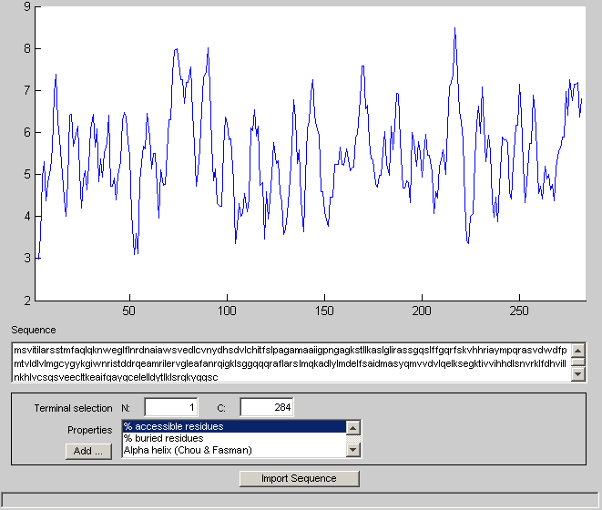
In the protein plot window, you must change the selected property to hydrophobicity (Kyte & Doolittle). Under Edit -> Change Configuration, you can also change the window size. Both profiles (original and filtered) are shown directly here for simplicity.

Sinteny

Here we analyze the synteny that is the relative order of genes on chromosomes. In other words, we must identify stretches where the relative ordering of orthologous genes has been conserved. The most intuitive manner to study sinteny is to construct a dot-plot. We simply line up all the genes in each genome according to their positions and plot only those for which the similarity score is above a certain threshold (here 110).

matrix=matrix(1:916,918:1965);
newermatrix=[matrix(:,751:end),matrix(:,1:750)];
[q,w]=find(newermatrix>110);
figure;
plot(q,w,'*')
title('ORF Sinteny Plot')
xlabel('C. Thrachomatis')
ylabel('C. Pneumoniae')

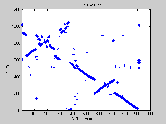
Observing the plot we notice that for the Chlamydia family there is almost complete synteny between the genomes. In fact the strong diagonal line shows that the genes with highest similarity are in corresponding positions. There are also two evident events of trasposition resulting in the two off-diagonals events.

Homologous intergenic regions and phylogenetic footprinting

Homologous intergenic regions are regions that evolve faster than the rest of the genome. The study of these is possible thanks to the synteny: genes are used as “anchors” to ensure that we are examining homologous intergenic sequence. Phylogenetic footprinting is a procedure based on such principle: anchoring the alignment with syntenic coding regions, conserved sequences can be individuted. Here we consider two 3-gene homologous synteny blocks of Chlamydia genomes.

t1=2253439;
t2=2252155;
t3=2253451;
t4=2253991;
t5=2254341;
t6=2255424;
t7=743266;
t8=746396;


bl1=joined(t2:t6);
bl2=joined(t7:t8);

We perform global alignment.

[sc,align]=nwalign(bl1,bl2);

vector=zeros(size(align(2,:)));
vector(strfind(align(2,:), '|'))=1;
vector(strfind(align(2,:), ':'))=0.1;

We plot the degree of conservation between the two sequences, using a moving window of size 75.

WS=75; %% windows size
for kk=1:length(vector)-WS
smoothvector(kk)=sum(vector(kk:kk+WS-1));
end

We define the function that shows the ORFs boundary.

oo=zeros(size(smoothvector));
oo(1:t1-t2)=0;
oo(t1-t2:t3-t2)=1;
oo(t3-t2:t4-t2)=0;
oo(t4-t2:t5-t2)=1;
oo(t6-t2:-1:t5-t2)=0;

figure;
plot(smoothvector)
hold on
plot(oo*(max(smoothvector)*1.1),'red')
title('Phylogenetic Footprint for three Chlamydia ORFs')
xlabel('Nucleotide Positions and ORF Boundaries')
ylabel('Degree of conservation')
hold off

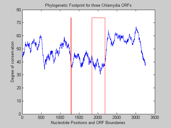
The plot shows that intergenic regions are less conserved than regions within ORFs.

Published with MATLAB® 7.1