DAUER Example of gene expression profile analysis

Introduction
Missing data
Cluster analysis
Principal Component Analysis
References

Introduction

It is known that gene expression in eukaryotes is regulated by transcription factor (TF) through binding to a short piece of DNA in the upstream region. With the emerging of large-scale gene expression and genomic sequence studies, one could identify by which transcription factors a certain gene is regulated and predict how the gene will act subjected to change of environment, based on the presence of TF binding sites in its upstream sequence. With the gene expression data, genes can be clustered on the basis of the similarity of their expression profiles and these clusters are likely to contain genes that are regulated by the same transcription factors. Searches for cis-regulatory elements can then be undertaken in the upstream regions of the clustered genes. In this example we identify the cis-regulatory elements present in the genes responsible to the dauer exit process in Caenorhabditis elegans. C. elegans is a small soil nematode found in temperate regions. The dauer is an important developmental transition in C. elegans that exhibits increased longevity, stress resistance, altered metabolism compared with normal worms. The transition from the dauer state to the non-dauer state is performed here by detecting significant change of expression profiles of genes between the two states. The temporal expression of genes are measured by microarray at 10 to 12 time points every one or two hours. In detail we have the expression profile of 1984 genes within 12 hours, sampled approximately once an hour. The data set can be obtained from Stanford Microarray Database:

web('http://cmgm.stanford.edu/~kimlab/dauer/ExtraData.htm');

You can load the data directly into the MATLAB workspace

load celegansdata.mat

You can verify the real number of genes in the data set. The cell array ‘genes’ contains the name of all genes.

numel(genes)

ans =

        1984

The information of one gene can be found by accessing the WormBase. Here you can also find the 1000bp upstream sequence corresponding to 1206 differentially expressed genes.

web('http://www.wormbase.org');

Let us analyze for example the gene F38E11.2 corresponding to the Heat Shock Protein.

genes{731}

web('http://www.wormbase.org/db/gene/gene?name=WBGene00002013;class=Gene');

ans =

F38E11.2

A plot shows the expression profile for this ORF

figure(1)
hold on
for i = 1:4
    plot(dauertime(dauerRep==i), degene(731, dauerRep==i))
end
hold off
xlabel('Time (Hours)')
ylabel('Log2 Relative Expression Level');

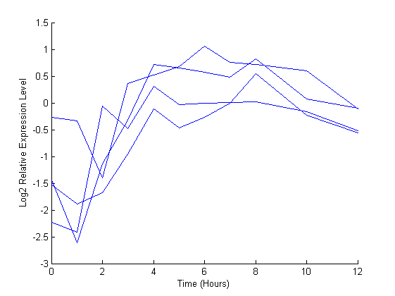
The gene associated with this ORF, hsp-12.6, appears to be up-regulated during the dauer exit.

Missing data

As frequently happens in this type of analysis, the original matrices used in that type of experiments have various entries with missing values. It is due to error of measurement or in the construction of the array. A possible approach to deal with this problem is to find the missing values using the MATLAB function isnan and than to replace those with the row medians.

missingVals = isnan(degene);
rowMedians = nanmedian(degene,2);
rowMed = repmat(rowMedians,1,size(degene,2));
degene(missingVals) = rowMed(missingVals);

Cluster analysis

The following in such analysis is the clustering of genes with respect to their temporal expression profiles. We decide to use the K-means clustering algorithm. As distance measure between the data points we consider d=1-corr, where corr indicates the sample correlation between two data points. The number of clusters must be set before executing the algorithm. To get the proper number of clusters we can perform hierarchical clustering and then visually inspect the heatmap. The MATLAB function clustergram perform hierarchical clustering and generate a heat map and dendrogram of the data. Here we adopt the simplest form of clustergram that clusters the rows of a data set using correlation as the distance metric and average linkage.

totalcluster = 10;
clustergram(degene,'colormap',jet,'symmetricrange',false,...
    'dendrogram',{'color',totalcluster});

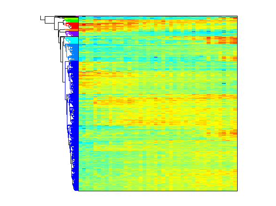
From the graphical display, six major groups can be seen. Based on this observation, we perform the K-means clustering by setting K = 6.

totalcluster = 6;
[cidx, ctrs] = kmeans(degene, totalcluster, 'dist','corr', 'rep',5,...
                                                        'disp','final');

34 iterations, total sum of distances = 409.21
21 iterations, total sum of distances = 409.21
37 iterations, total sum of distances = 409.123
20 iterations, total sum of distances = 412.756
19 iterations, total sum of distances = 409.391

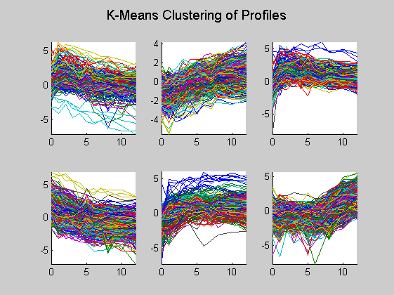
Here in each plot the gene profiles in the same cluster are plotted together.

figure
for c = 1:totalcluster
    subplot(2,3,c);
    hold on
    for i = 1:4
        plot(dauertime(dauerRep==i),degene((cidx == c),dauerRep == i)');
    end
    hold off
    axis tight
end
suptitle('K-Means Clustering of Profiles');

Then only the centroid profiles are plotted for each cluster so that the expression pattern can be examined more clearly.

figure
for c = 1:totalcluster
    subplot(2,3,c);
    hold on
    for i = 1:4
        plot(dauertime(dauerRep==i),ctrs(c, dauerRep==i)');
    end
    hold off
    axis tight
end
suptitle('K-Means Clustering of Centroid Profiles');

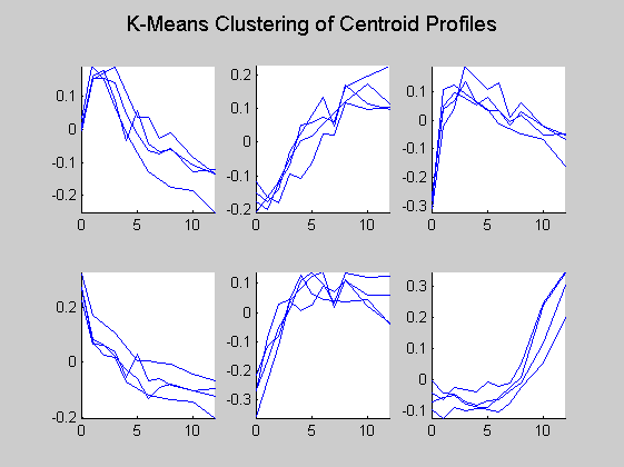
Cluster 6 represents the genes that are up-regulated at late stage during the process. Genes in cluster 3 have sharp increase at the beginning but slowly decrease toward the end of the process. Cluster 1 shows the pattern of slightly increase at the beginning followed by gradual drop down. Cluster 2 contains genes with steady increase during the whole process. Cluster 4 shows sharp decrease at the beginning, followed by slowly decrease. Genes in Cluster 5 increase sharply at the beginning, and then reach the plateau.

The motifs of genes with similar expression pattern are then searched within each cluster. The Expectation Maximization algorithm has been used for that aim.

addpath ./motif/;
[names, seqs, priors] = load_seqs('seq1984.fasta', 1);
shortnames = strtok(names, ' (');
shortcidx = [];

for i = 1:length(shortnames)
  x = find(strcmp(genes, shortnames{i}));
  if length(x)~=0, shortcidx(i) = cidx(x); end;
end

for c = 1:totalcluster
  subseqs = seqs((shortcidx==c),:);
  winsize = 10;
  bg_model = build_uniform_motif_model(1);
  motif_model = build_uniform_motif_model(winsize);
  pcounts = repmat(0.25, 4, winsize);
  num_motifs = 5;
  [final_matrices, final_bgs] = em(subseqs, priors, bg_model, motif_model, ...
    pcounts, num_motifs, 1);
end

Motif 1: ==> TTTTTTTTTC

Motif 2: ==> AAAAAAAAAA

Motif 3: ==> CCGCCTCCCC

Motif 4: ==> GAAAAATTGG

Motif 5: ==> TTCATTTTTC

Motif 1: ==> TTTTTTTTTC

Motif 2: ==> GAAAAAAAAA

Motif 3: ==> CCTTTTTTCC

Motif 4: ==> GAAAAAAAAA

Motif 5: ==> CAATTTTTTG

Motif 1: ==> TTTTTTTTTC

Motif 2: ==> CAAAAAAAAA

Motif 3:==> CCCCTCCCCC

Motif 4: ==> GAAAAATTGG

Motif 5: ==> TTTTTTTTTT

Motif 1: ==> TTTTTTTTTT

Motif 2: ==> GAAAAAAAAA

Motif 3: ==> CCCCCCCCCC

Motif 4: ==> GAAAAATTGG

Motif 5: ==> CAATTTTTTC

Motif 1: ==> TTTTTTTTTC

Motif 2: ==> AAAAAAAAAA

Motif 3: ==> CTTCCCCCCC

Motif 4: ==> GAAAAATTTG

Motif 5: ==> TTTTTTTTTC

Motif 1: ==> TTTTTTTTTC

Motif 2: ==> AAAAAAAAAA

Motif 3: ==> CCCCCCCCCC

Motif 4: ==> AAAAATTTTT

Motif 5: ==> GAAAAAGAAA

Some of the motifs are present in almost all clusters, for example, TTTTTTTTTC and AAAAAAAAAA, and some motifs are present multiple times in the same cluster. These may due to the redundant sequences in the genome. They are often found out first probably because their frequent appearance in the genome. Therefore, the redundant sequence should be masked for the subsequent search. The rest are unique to the cluster.

Principal Component Analysis

Timing of up or down regulation of genes accurately is important to the developmental process. Principal component analysis is carried out to examine the temporal variation.

[pc, zscores, pcvars] = princomp(degene);
pcvars./sum(pcvars) * 100;
cumsum(pcvars./sum(pcvars) * 100)

The first two components take into account more than 70% of the total variation. The MATLAB function gscatter creates a grouped scatter plot, where the group is created by clusterdata function. The genes fo each group are identified also by names.

figure
pcclusters = clusterdata(zscores(:,1:2),'maxclust',6,'linkage','av');
gscatter(zscores(:,1),zscores(:,2),pcclusters)
xlabel('First Principal Component');
ylabel('Second Principal Component');
title('Principal Component Scatter Plot with Colored Clusters');

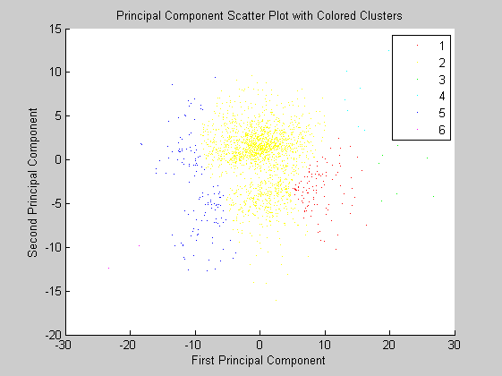
The first principal component represents variation approximately along the slope of increase, while the second is rather flat probably representing the variation of intercepts

References

J. Wang, S. K. Kim. Global Analysis of Gene Expression in the Dauer Larvae of Caenorhabditis elegans. Development 130:
1621-1634, 2003