HIV Example of quantitative analysis of natural selection.

Contents

Introduction

In 1983 the infectious agent responsible of the well-known disease of Acquired Immune Deficiency Syndrome (AIDS) was identified. It was called Human Immunodeficiency Virus (HIV). Despite this discovery of fundamental importance, at the present there is no cure for this disease and no effective vaccine against HIV infection. The main difficulty is that our immune system as well as any drugs cannot deal with the inner nature of this virus that evolves constantly and rapidly. The genome of HIV has been sequenced hundreds of time since the eighties, so it is possible to study the differences between many individual genomes. This can help us to gain a general understanding of how virus evolves. In particular there are specific regions of its proteins that are recognized and attacked by our immune system: these regions mostly show the signature of adaptive evolution of the changing virus. Other regions instead remain invariant having important biological functions and not being involved in interactions with the immune system. In this example a genome wide analysis of natural selection in HIV is performed.

ORF Finding

The HIV genome has nine ORFs but 15 proteins are made in all (some genes are translated into large polyproteins which are then cleaved by a virus-encoded protease into smaller proteins). Some ORFs overlap slightly and there are also some introns. All this factor complicate the detection of genes. Let’s consider for example a sequence of an HIV genome. It can be downloaded from the GenBank database with the MATLAB function getgenbank.

hiv=getgenbank('NC_001802','SequenceOnly',true);

You can also download directly the .mat file here.

%load hiv

The simplest algorithm to find ORFs in this sequence consists in selecting the statistically significant ORFs between all those found by the function seqorfs

 [orf n]=seqorfs(hiv,'MINIMUMLENGTH',1);

Following this approach a single-nucleotide permutation test on the sequence is performed to determine a threshold of minimum length for an ORF to be considered gene. The threshold is chosen in order to keep as candidate genes all ORFs of length equal to or greater than the top 5% of random ORFs.

[orfr nr]=seqorfs(hiv(randperm(length(hiv))),'MINIMUMLENGTH',1);
ORFLengthr=[];
for i=1:6
    ORFLengthr=[ORFLengthr; orfr(i).Length'];
end
empirical_threshold=prctile(ORFLengthr,95)
[orf n]=seqorfs(hiv,'MINIMUMLENGTH',empirical_threshold/3);

empirical_threshold =

  159.3000

The informations associated with the detected ORFs can be saved in an array and shown for all the reading frames of the positive strand.

HIV_ORF=[];
for i=1:3
    HIV_ORF=[HIV_ORF; orf(i).Start' orf(i).Stop' orf(i).Length' orf(i).Frame'];
end
HIV_ORF

HIV_ORF =

        3955        4120         165           1
        5377        5593         216           1
        5608        5854         246           1
        1904        4640        2736           2
        5105        5339         234           2
        5771        8339        2568           2
         336        1836        1500           3
        4587        5163         576           3
        8343        8712         369           3

Note that there are more genes in the HIV genome, but some protein-coding regions are missed because of the semplicity of the algorithm. Hidden Markov Model should be used for that.

Ka/Ks

The Ka/Ks ratio is a measure, introduced by the Japanese Kimura, of natural selection, comparing the number of non-synonimous to synonymous substitutios in a gene. Here we compute the Ka/Ks ratio for the genes of two different sequences of HIV-1 (Genbank accession numbers AF033819 and M27323).

hiv1_all=getgenbank('AF033819');

hiv1=hiv1_all.Sequence;

hiv2_all=getgenbank('M27323');

hiv2=hiv2_all.Sequence;

As before, you can also download directly the .mat file here.

%load hivcomparison

We must compare corresponding protein sequence. Therefore is necessary to individuate corresponding regions in the sequence. The field Features of the structures can be used for that purpose.

%      GAG POL VIF VPX/VPU VPR TAT REV ENV  NEF
% seq1  1   2   3     7     4   5   6   8    9
% seq2  1   2   3     7     4   5   6   8    9

ind1=[1 2 3 7 4 5 6 8 9];
ind2=[1 2 3 7 4 5 6 8 9];

for ind=1:9
        temp_seq =hiv1;
        CDSs = hiv1_all.CDS;
        seq1= temp_seq(CDSs(ind1(ind)).indices(1):CDSs(ind1(ind)).indices(2));
        g1(ind).Sequence = seq1(str2num(CDSs(ind1(ind)).codon_start):end);
        temp_seq = hiv2;
        CDSs = hiv2_all.CDS;
        seq2= temp_seq(CDSs(ind2(ind)).indices(1):CDSs(ind2(ind)).indices(2));
        g2(ind).Sequence = seq2(str2num(CDSs(ind2(ind)).codon_start):end);
end

After aligning the corresponding ORFs, the Ka/Ks ratio can be calculated.

for i=1:9
        [sc,alig]= nwalign(nt2aa(g1(i).Sequence),nt2aa(g2(i).Sequence));
        seq1 = seqinsertgaps(g1(i).Sequence,alig(1,:));
        seq2 = seqinsertgaps(g2(i).Sequence,alig(3,:));
        %Calculate synonymous and nonsynonymous substitution rates.
        [dn,ds] = dnds(seq1,seq2);
        KaKs(i)=dn/ds;
end

KaKs

KaKs =

    0.2357    0.1235    0.2758    0.4749    0.1042    1.0516    0.1813    0.4723    0.3043

The ENV gene

For the analysis of single genes is convenient to calculate the Ka/Ks ratio locally (using for example a sliding window) instead of averaging its value over the entire gene. For example, in this case we study the ENV gene. This gene codes for the envelope glycoprotein gp160, which is a precursor to two proteins: gp41 and gp120. In particular, the last one is responsible of two important processes: to maintain continously recognition of host cells and simultaneously to avoid detection by the immune system. These roles are carried out by different parts of the gp120 protein, therefore measuring the global Ka/Ks ratio obscures both processes. It is necessary to measure the effect of selection on smaller region of the gene, by computing Ka/Ks in sliding windows.

   env1 = g1(8).Sequence;
   env2 = g2(8).Sequence;

  [sc,alig] = nwalign(nt2aa(env1),nt2aa(env2));

  seq1 = seqinsertgaps(env1,alig(1,:));
  seq2 = seqinsertgaps(env2,alig(3,:));
  S=[seq1; seq2];

The following plots the local Ka/Ks ratio with a sliding window of 60 codons. The blue line shows the Ks values, the red one the Ka values and the green the ratio KaKs.

  KaKs_ratio_WL(S,60);
  title('Sliding window analysis - ENV protein');

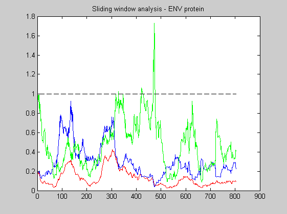
As expected the rate of non-synonymous substitution is greater than the rate of synonimous ones. These region are clearly recognized by the human immune system. There are also many regions with Ka/Ks less than one: they corresponds to regions necessary to the virus to recognize the receptors of its host cells. From the plot it is also evident that the average ratio for the entire gene is less than one. As a confirm we can calculate it.

 [dn ds vardn vards] = dnds(seq1, seq2);
 KaKs=dn/ds

KaKs =

    0.4723

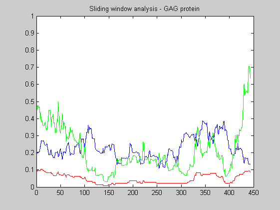
GAG Polyprotein

The same analysis of above can be repeated for the GAG polyprotein. GAG is another genes common to all the retroviruses. It contains around 1500 nucleotides and encodes four different proteins wich form the building block for the viral core. This protein contain additional epitopes recognized by the human himmune system, and hence it is under constant pressure to escape by evolving.

   gag1 = g1(1).Sequence;
   gag2 = g2(1).Sequence;


  [sc,alig] = nwalign(nt2aa(gag1),nt2aa(gag2));
  seq1 = seqinsertgaps(gag1,alig(1,:));
  seq2 = seqinsertgaps(gag2,alig(3,:));
  S=[seq1; seq2];

  KaKs_ratio_WL(S,60);
  title('Sliding window analysis - GAG protein');

Published with MATLAB® 7.1