HAEMOPHILUS Example of sequence statistics and gene finding with MATLAB
This demonstration looks at some statistics about the DNA content of the Haemophilus Influenzae. It shows also some algorithms for finding ORFs and for assessing their significance.
Contents
Introduction
Haemophilus influenzae is a non-motile Gram-negative coccobacillus first described in 1892 by Dr. Robert Pfeiffer during an influenza pandemic. It is generally aerobic, but can grow as a facultative anaerobe. It is responsible for a wide range of clinical diseases. The Haemophilus influenzae genome was the first to be sequenced and assembled in a free-living organism. It contains about 1.8 million base pairs and is estimated to have 1,740 genes.
Accessing NCBI data from the MATLAB workspace
The dna sequence can be obtained from the GenBank database with the accession number NC_000907. Using the getgenbank function with the ‘SequenceOnly’ flag just the nucleotide sequence is loaded into the MATLAB workspace.
Hflu = getgenbank('NC_000907','SequenceOnly',true);
If you don’t have a live web connection, you can load the data from a MAT-file using the command
% load Hflu % <== Uncomment this if no internet connection
The MATLAB whos command gives information about the size of the sequence.
whos Hflu
  Name       Size                    Bytes  Class

  Hflu       1x1830138             3660276  char array

Grand total is 1830138 elements using 3660276 bytes
The total length of the Haemophilus Influenzae genome is 1830138 bp.
Statistical sequence analysis
You will examine some statistics properties of the sequence. You can look at the composition of the nucleotides with the basecount function.
bases=basecount(Hflu)
Warning: Ambiguous symbols 'NKRNNRNSSNYKMMRSYNNNNYKNNNNSYWNMMMNKWNWYNNNSMRNNWNNWMKKNMYKNNKNYWRNKKSWNNNSSNNNNWYWSNNNYKNNRNRSSRMKRKMSKMNNWNWNYRYN' appear in the sequence. These will be in Others.

bases =

         A: 567623
         C: 350723
         G: 347436
         T: 564241
    Others: 115
The four nucleotides are not used at equal frequency across the genome: A and T are much common than G and C.
Others symbols occur in the sequence. They correspond to positions in the sequence that are are not clearly one base or another and they are due, for example, to sequencing uncertainties. In this case for example: N: aNy base –
K: G or T –
R: A or G (puRine) –
Y: C or T (pYrimidine) –
M: A or C (aMino) –
S: C or G –
W: A or T.
Instead of grouping other simbols together, you can count them individually.
bases=basecount(Hflu,'Others','Full')
bases =

      A: 567623
      C: 350723
      G: 347436
      T: 564241
      R: 10
      Y: 11
      K: 14
      M: 11
      S: 12
      W: 11
      B: 0
      D: 0
      H: 0
      V: 0
      N: 46
    Gap: 0
You can also calculate the frequency of each nucleotide.
[bases frequency]=basecountfrequency(Hflu,'Others','Full')
bases =

      A: 567623
      C: 350723
      G: 347436
      T: 564241
      R: 10
      Y: 11
      K: 14
      M: 11
      S: 12
      W: 11
      B: 0
      D: 0
      H: 0
      V: 0
      N: 46
    Gap: 0


frequency =

      A: 0.3102
      C: 0.1916
      G: 0.1898
      T: 0.3083
      R: 5.4641e-06
      Y: 6.0105e-06
      K: 7.6497e-06
      M: 6.0105e-06
      S: 6.5569e-06
      W: 6.0105e-06
      B: 0
      D: 0
      H: 0
      V: 0
      N: 2.5135e-05
    Gap: 0
It should be pointed out that these are on the 5′-3′ strand of DNA, but we know exactly the frequency of all the the bases on the other strand because of the complementarity of the double helix. Anyway we could verify it using again the basecountfrequency function.
[bases frequency]=basecountfrequency(seqrcomplement(Hflu),'Others','Full')
bases =

      A: 564241
      C: 347436
      G: 350723
      T: 567623
      R: 11
      Y: 10
      K: 11
      M: 14
      S: 12
      W: 11
      B: 0
      D: 0
      H: 0
      V: 0
      N: 46
    Gap: 0


frequency =

      A: 0.3083
      C: 0.1898
      G: 0.1916
      T: 0.3102
      R: 6.0105e-06
      Y: 5.4641e-06
      K: 6.0105e-06
      M: 7.6497e-06
      S: 6.5569e-06
      W: 6.0105e-06
      B: 0
      D: 0
      H: 0
      V: 0
      N: 2.5135e-05
    Gap: 0
CG content
The local fluctuations in the frequencies of nucleotides provide different interesting information. The local base composition by a sliding window of variable size can be measured. In the following the window size is assumed 90000 bp and 20000 bp respectively.
ntdensity1(Hflu,'window',90000)
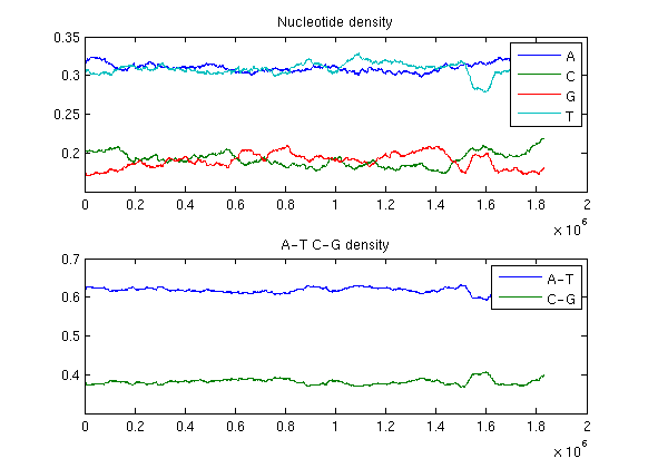
ntdensity1(Hflu,'window',20000)
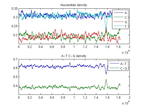
The phenomenon called horizontal gene transfer can be observed in the second plot: the H. influenzae genome contains a 30Kb region of unusual GC content from 1.56Mb to 1.59Mb.
k-mer frequency and motif bias
Now look at the dimers in the sequence and display the 2-mer frequencies in the table matrix. The simbols others than A, C, G, T are not considered.
[dimers,matrix] = dimercount(Hflu)
Warning: Ambiguous symbols 'NKRNNRNSSNYKMMRSYNNNNYKNNNNSYWNMMMNKWNWYNNNSMRNNWNNWMKKNMYKNNKNYWRNKKSWNNNSSNNNNWYWSNNNYKNNRNRSSRMKRKMSKMNNWNWNYRYN' appear in the sequence. These will be in Others.

dimers =

        AA: 219880
        AC: 92410
        AG: 88457
        AT: 166837
        CA: 121618
        CC: 68014
        CG: 72523
        CT: 88551
        GA: 94125
        GC: 95529
        GG: 66448
        GT: 91314
        TA: 131955
        TC: 94745
        TG: 119996
        TT: 217512
    Others: 223


matrix =

    0.1202    0.0505    0.0483    0.0912
    0.0665    0.0372    0.0396    0.0484
    0.0514    0.0522    0.0363    0.0499
    0.0721    0.0518    0.0656    0.1189
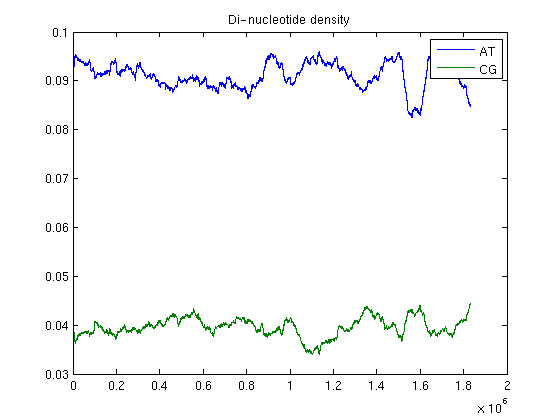
You can also plot the frequency of certain di-nucleotides of interest: for example considering the local fluctuations in the frequencies of dimers AT and CG.
density = dndensity(Hflu)
As a further analysis you can also compare the observed frequency of each dimer with the one expected under the multinomial model. This is called genome signature.
gs=gensign(Hflu)
Warning: Ambiguous symbols 'NKRNNRNSSNYKMMRSYNNNNYKNNNNSYWNMMMNKWNWYNNNSMRNNWNNWMKKNMYKNNKNYWRNKKSWNNNSSNNNNWYWSNNNYKNNRNRSSRMKRKMSKMNNWNWNYRYN' appear in the sequence. These will be in Others.
Warning: Ambiguous symbols 'NKRNNRNSSNYKMMRSYNNNNYKNNNNSYWNMMMNKWNWYNNNSMRNNWNNWMKKNMYKNNKNYWRNKKSWNNNSSNNNNWYWSNNNYKNNRNRSSRMKRKMSKMNNWNWNYRYN' appear in the sequence. These will be in Others.

gs =

    1.2491    0.8496    0.8210    0.9535
    1.1182    1.0121    1.0894    0.8190
    0.8736    1.4349    1.0076    0.8526
    0.7541    0.8763    1.1204    1.2505
You can look at codons using codoncount. That function counts the codons on a particular reading frame. With no options, the function shows the codon counts on the first reading frame.
codoncount(Hflu)
Warning: Ambiguous symbols 'NKRNNRNSSNYKMMRSYNNNNYKNNNNSYWNMMMNKWNWYNNNSMRNNWNNWMKKNMYKNNKNYWRNKKSWNNNSSNNNNWYWSNNNYKNNRNRSSRMKRKMSKMNNWNWNYRYN' appear in the sequence. These will be in Others.
AAA - 27760     AAC - 11523     AAG - 11701     AAT - 22178
ACA -  9121     ACC -  7249     ACG -  6917     ACT -  7801
AGA -  8763     AGC -  8142     AGG -  5340     AGT -  7569
ATA - 12768     ATC - 11041     ATG - 10029     ATT - 22007
CAA - 15527     CAC -  7692     CAG -  6634     CAT - 10049
CCA -  9185     CCC -  3866     CCG -  4213     CCT -  5502
CGA -  6311     CGC -  6771     CGG -  4112     CGT -  7255
CTA -  6110     CTC -  4112     CTG -  6625     CTT - 11985
GAA - 12946     GAC -  3624     GAG -  4202     GAT - 10719
GCA - 10832     GCC -  6310     GCG -  6537     GCT -  8153
GGA -  5296     GGC -  6218     GGG -  3590     GGT -  7147
GTA -  7714     GTC -  3651     GTG -  7741     GTT - 11118
TAA - 16924     TAC -  7723     TAG -  6372     TAT - 12561
TCA - 11592     TCC -  5542     TCG -  6240     TCT -  8663
TGA - 11513     TGC - 10991     TGG -  9045     TGT -  9079
TTA - 17139     TTC - 12550     TTG - 15162     TTT - 27184
Others - 110
Exploring the Open Reading Frames (ORFs)
In a nucleotide sequence an obvious thing to look for is if there are any open reading frames. The function seqorfs can be used to determine the ORFs in a sequence.
orf=seqorfs(Hflu);
The variable orf is a structure with information about the start/stop positions of each ORFs, its length and which reading frame it is in. Here the minimun number of codons for an ORF to be considered valid is 10 (default value).
The minimun number of codons for an ORF to be considered valid can be also set. Here a threshold of 70 and 80 amino acids are considered leading to about 2175 and 1966 ORFs respectively.
[orf n_70]=seqorfs(Hflu,'MINIMUMLENGTH',70);

n_70
n_70 =

        2175
[orf n_80]=seqorfs(Hflu,'MINIMUMLENGTH',80);

n_80
n_80 =

        1966
You can also look for the total number of ORFs
[orf n]=seqorfs(Hflu,'MINIMUMLENGTH',1);

n
n =

       37500
Detecting significant ORFs
The classic approach to decide whether an ORF is a good candidate as a gene is to calculate the probability of seeing an ORF of a certain length L in a random sequence. To test the significance of ORFs a single-nucleotide permutation test can be used.
[orf1 n1]=seqorfs(Hflu(randperm(length(Hflu))),'MINIMUMLENGTH',1);

n1
n1 =

       52174
The ORF Length of the original and of the randomized sequences can be compared.
ORFLength=[];
for i=1:6
    ORFLength=[ORFLength; orf(i).Length'];
end

ORFLength1=[];
for i=1:6
    ORFLength1=[ORFLength1; orf1(i).Length'];
end
A threshold must be chosen in order to keep as candidate genes those ORFs in the H. Influenzae genome that are longer than most (or all) the ORFs in the random sequence.
max_threshold=max(ORFLength1)

n_max=length(find(ORFLength>=max_threshold))
max_threshold =

   573


n_max =

        1182
You can also use a more tolerant threshold in order to keep all ORFs of length equal to or greater than the top 1% of random ORFs.
empirical_threshold=prctile(ORFLength1,99)
n_emp=length(find(ORFLength>=empirical_threshold))
empirical_threshold =

   207


n_emp =

        2209